The Two-Asset Household with Sequential EGM - The Sequential Endogenous Grid Method

This notebook solves the two-asset liquid-illiquid household block of Section 3 at the published calibration of Auclert et al. (2021). It walks through the closed-form illiquid inversion, solves the household to its stationary policies, draws the endogenous mesh the inversion produces, and reruns one row of the paper’s comparison with the nested method (NEGM).

import sys

sys.path.append("../")
sys.path.append("../figures")

import matplotlib.pyplot as plt
import numpy as np
from cli import format_table
from figure_styles import apply_engine_style
from generate_grid_transformation_abrs import (
    draw_grid_transformation,
    get_two_asset_meshes,
)
from matplotlib.colors import TwoSlopeNorm
from repo_paths import FIG_DIR, read_rows
from ssj.bench_accuracy_negm import accuracy_row
from ssj.benchmark import (
    assert_mesh_fold_free,
    assert_mesh_ipm,
    budget_violation,
    calibration,
    l_grid_for,
    solve_compact,
    solve_negm,
    stage0_mesh,
)
from ssj.hh_egm import psi_and_derivs, stage0_node

apply_engine_style()

1The Household Problem¶

A household enters the period with liquid wealth $b$ , an illiquid balance $a$ and productivity $e$ , which follows a three-state Markov chain. Out of market resources $m = R_{b} b + R_{a} a + y (e)$ it chooses consumption $c$ and new balances $b^{'} \geq 0$ , $a^{'} \geq 0$ subject to

c + b^{'} + a^{'} + Ψ (a^{'}, a) = m, Ψ (a^{'}, a) = \frac{χ_{1}}{2} {(\frac{a^{'} - R_{a} a}{R_{a} a + χ_{0}})}^{2} (R_{a} a + χ_{0}) .

(1)

The illiquid asset pays the higher return, but moving funds into or out of it incurs the convex cost $Ψ$ . Every two-asset exhibit in the paper uses the calibration below. The table computes relative risk aversion as the inverse of the elasticity of intertemporal substitution, which the code stores.

cal = calibration(40, 60)
print(format_table(
    ["Parameter", "Value"],
    [
        ["Discount factor (beta)", cal["beta"]],
        ["Relative risk aversion (rho)", 1 / cal["eis"]],
        ["Liquid return (r_b)", cal["rb"]],
        ["Illiquid return (r_a)", cal["ra"]],
        ["Cost offset (chi_0)", cal["chi0"]],
        ["Cost scale (chi_1)", cal["chi1"]],
        ["Productivity persistence", cal["rho_z"]],
        ["Productivity dispersion", cal["sigma_z"]],
        ["Largest liquid node", cal["bmax"]],
        ["Largest illiquid node", cal["amax"]],
    ],
))

Parameter                     Value
----------------------------  ------
Discount factor (beta)        0.976
Relative risk aversion (rho)  2.0
Liquid return (r_b)           0.0075
Illiquid return (r_a)         0.0125
Cost offset (chi_0)           0.25
Cost scale (chi_1)            6.5
Productivity persistence      0.966
Productivity dispersion       0.92
Largest liquid node           50.0
Largest illiquid node         4000.0

2The Illiquid Stage in Closed Form¶

The period splits into an illiquid choice (Stage 0), a consumption choice (Stage 1) and the expectation over next period’s productivity. Stage 1 is the standard consumption EGM at each fixed $a^{'}$ . It leaves liquid resources $ℓ = m - a^{'} - Ψ (a^{'}, a)$ as the state of Stage 0, whose first-order condition is

1 + Ψ_{1} (a^{'}, a) = \frac{v_{a^{'}}^{1} (ℓ, a^{'}, e)}{v_{ℓ}^{1} (ℓ, a^{'}, e)} .

(2)

Nested methods search for the $a^{'}$ that solves this equation at each state. EGM $^{n}$ fixes $a^{'}$ on a grid and solves for the incoming balance $a$ instead. With the quadratic cost, $Ψ_{1} = χ_{1} u$ for the adjustment rate $u = (a^{'} - R_{a} a) / (R_{a} a + χ_{0})$ , so the wedge $τ = v_{a^{'}}^{1} / v_{ℓ}^{1} - 1$ inverts in two lines:

u^{*} = \frac{τ}{χ_{1}}, a = \frac{a^{'} - u^{*} χ_{0}}{R_{a} (1 + u^{*})} .

(3)

At every node of the $(ℓ, a^{'})$ grid, the solver applies stage0_node. One call at illustrative inputs shows that the incoming balance it returns satisfies the first-order condition.

Ra, Rb = 1 + cal["ra"], 1 + cal["rb"]
chi0, chi1, chi2 = cal["chi0"], cal["chi1"], cal["chi2"]

v1_ap, c, a_prime, ell = 0.9, 1.2, 3.0, 5.0  # Stage 1 outputs at one node
tau = v1_ap * c ** (1 / cal["eis"]) - 1  # v1_ap / u'(c) - 1
a_in, b_in = stage0_node(
    v1_ap, c, a_prime, ell, cal["z"][1], 1 / cal["eis"], Ra, Rb, chi0, chi1, chi2
)
_, psi1, _ = psi_and_derivs(a_prime, a_in, Ra, chi0, chi1, chi2)
print(f"incoming balances: a = {a_in:.6f}, b = {b_in:.6f}")
print(f"Psi_1(a', a) = {psi1:.15f}")
print(f"wedge tau    = {tau:.15f}")

incoming balances: a = 2.823157, b = 4.456302
Psi_1(a', a) = 0.296000000000001
wedge tau    = 0.296000000000000

Up to rounding error, the marginal cost $Ψ_{1}$ equals the wedge $τ$ . The incoming liquid balance $b$ then follows from the two accounting identities, with no root-finding or iteration at any step.

3Solving the Household¶

solve_compact iterates the EGM $^{n}$ backward step from the initial marginal values of the sequence-space Jacobian toolkit until the marginal values change by less than 10^-9, the tolerance of every published solve. It raises an error if the iteration does not converge.

egmn = solve_compact(cal)
print(f"EGM^n converged in {egmn['iter']} iterations")
print(f"largest budget residual: {budget_violation(egmn, cal).max():.1e}")
adjustment = np.abs(egmn["a"] - (1 + cal["ra"]) * cal["a"][None, None, :])
print(f"median illiquid adjustment |a' - R_a a|: {np.median(adjustment):.3f}")

EGM^n converged in 395 iterations
largest budget residual: 9.1e-13
median illiquid adjustment |a' - R_a a|: 0.338

The delivered policies satisfy the within-period budget to rounding error at every node, because the liquid choice is the budget residual.

The Liquid-Resources Grid¶

Stage 0 receives the Stage 1 policies on a regular grid of liquid resources $ℓ$ , which must cover every $ℓ$ the inversion can request. A household rich in illiquid wealth can withdraw to finance liquidity, so liquid wealth alone does not bound that range. Since the marginal value of illiquid wealth is non-negative, the first-order condition caps the withdrawal and with it $ℓ$ , at

ℓ = R_{b} b + y + \frac{R_{a} a + χ_{0}}{2 χ_{1}},

(4)

well past the largest liquid node. The solver builds its $ℓ$ -grid to this bound:

l_grid = l_grid_for(cal)
ell_bar = Rb * cal["b"][-1] + cal["z"].max() + (Ra * cal["a"][-1] + chi0) / (2 * chi1)
print(f"largest liquid node:      {cal['b'][-1]:.2f}")
print(f"closed-form bound:        {ell_bar:.2f}")
print(f"largest l-grid node:      {l_grid[-1]:.2f}")
print(f"l-grid nodes past b-grid: {l_grid.size - cal['b'].size}")

largest liquid node:      50.00
closed-form bound:        364.40
largest l-grid node:      364.40
l-grid nodes past b-grid: 10

4The Endogenous Mesh¶

The inversion maps the exogenous $(ℓ, a^{'})$ grid into a curvilinear mesh of incoming states $(b, a)$ . ENGINE interpolates on that mesh only if it is fold-free (no cell turns inside out) and index-monotone (each coordinate increases along its own grid index). The paper verifies both on every reported mesh. Here the same checks run on the converged $40 \times 60$ solution:

mesh = stage0_mesh(egmn, cal)
assert_mesh_fold_free(mesh["b_endo"], mesh["a_endo"])
assert_mesh_ipm(mesh["b_endo"], mesh["a_endo"])
print("Fold-free and index-monotone in all", mesh["a_endo"].shape[0], "productivity states")

Fold-free and index-monotone in all 3 productivity states

Each check raises an error on the first violation it finds.

Below, the paper’s grid-transformation figure is redrawn on its own $20 \times 20$ grid, where individual mesh lines stay visible.

fig = draw_grid_transformation(get_two_asset_meshes())
plt.show()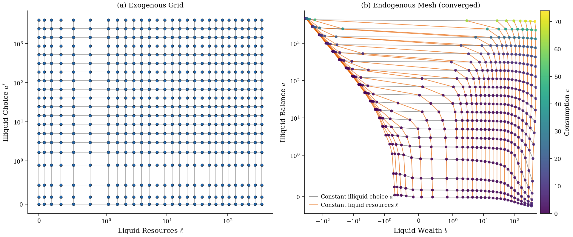

Where the optimal adjustment is largest, the inversion bends the mesh most. Lines of constant $ℓ$ and constant $a^{'}$ never cross. Nodes with negative $b$ belong to withdrawal-financed choices outside the state space; the regrid to the regular $(b, a)$ grid never queries them.

The Adjustment Wedge¶

Every backward step produces the Stage 1 marginal values on the whole $(ℓ, a^{'})$ grid, and with them the wedge $τ$ : the shadow price, in units of liquid wealth, of moving one unit into the illiquid account. It follows from the inverted mesh through $τ = χ_{1} u$ :

ie = cal["Pi"].shape[0] // 2  # median productivity state
a_endo = mesh["a_endo"][ie]
u = (cal["a"][None, :] - Ra * a_endo) / (Ra * a_endo + chi0)
L, AP = np.meshgrid(l_grid, cal["a"], indexing="ij")

tau_grid = chi1 * u
fig, ax = plt.subplots(figsize=(7, 5))
pc = ax.pcolormesh(L, AP, tau_grid, cmap="RdBu_r", norm=TwoSlopeNorm(0.0), shading="auto")
ticks = [-1.0, -0.5, 0.0, *np.arange(10.0, tau_grid.max(), 10.0)]
fig.colorbar(pc, ax=ax, label=r"Wedge $\tau$", ticks=ticks)
ax.set_xscale("symlog", linthresh=1.0)
ax.set_yscale("symlog", linthresh=1.0)
ax.set_xlabel(r"Liquid Resources $\ell$")
ax.set_ylabel(r"Illiquid Choice $a'$")
plt.show()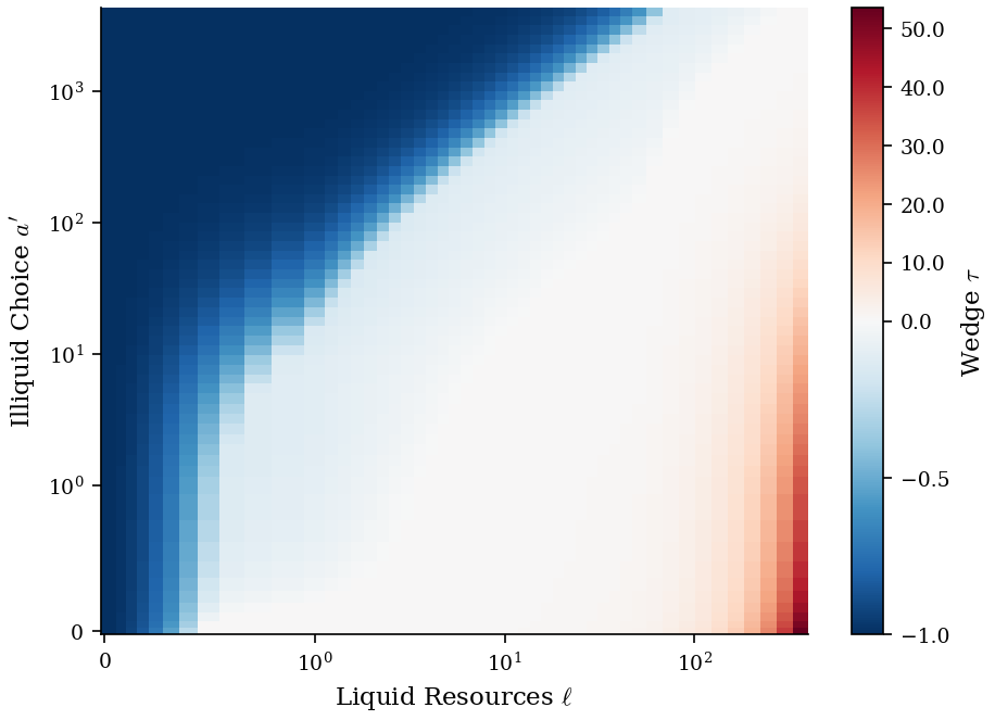

Households with ample liquid resources and a small illiquid position deposit at the largest rates (lower right). Where liquid resources are scarce relative to the illiquid choice, the marginal value of liquidity swamps that of the illiquid account. There the wedge approaches its lower bound of -1, which it attains at $ℓ = 0$ .

5Policy Functions¶

Consumption, the liquid choice and the net illiquid deposit $a^{'} - R_{a} a$ on the regular $(b, a)$ grid, at the median productivity state and the four illiquid grid nodes nearest 0, 10, 100 and 1000:

ia_show = [int(np.argmin(np.abs(cal["a"] - a0))) for a0 in (0.0, 10.0, 100.0, 1000.0)]
policies = {
    "Consumption $c$": egmn["c"][ie],
    "Liquid choice $b'$": egmn["b"][ie],
    "Net deposit $a' - R_a a$": egmn["a"][ie] - Ra * cal["a"][None, :],
}
fig, axes = plt.subplots(1, 3, figsize=(15, 4.5))
for ax, (title, policy) in zip(axes, policies.items(), strict=True):
    for ia in ia_show:
        ax.plot(cal["b"], policy[:, ia], label=f"$a = {cal['a'][ia]:.0f}$")
    ax.set_xlabel("Liquid wealth $b$")
    ax.set_title(title)
axes[0].legend()
plt.tight_layout()
plt.show()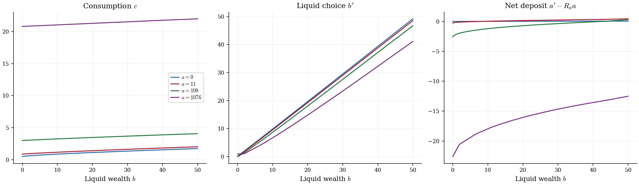

Holding $a$ fixed, more liquid wealth raises consumption and the liquid choice. The two larger illiquid balances fund part of their spending by withdrawing from the illiquid account, most heavily when liquid wealth is low. At the lowest $b$ , the largest balance withdraws enough to carry some of it into liquid savings, so its $b^{'}$ starts above the others.

6Comparison with the Nested Method¶

NEGM shares every stage with EGM $^{n}$ except Stage 0, where it solves the first-order condition at each regular-grid node by a safeguarded bracketing iteration. accuracy_row writes each row of the archive’s accuracy_negm.csv. Run here on both solutions at the $(40, 60)$ timing grid, its output is shown beside the published row.

negm = solve_negm(cal)
grid = (len(cal["b"]), len(cal["a"]))
row = accuracy_row("timing", grid, cal, egmn, negm)
published = next(
    r
    for r in read_rows(FIG_DIR / "accuracy_negm.csv")
    if (r["family"], int(r["nB"]), int(r["nA"])) == ("timing", *grid)
)
print(format_table(
    ["Column", "This run", "Published"],
    [[k, v, published[k]] for k, v in zip(published, row, strict=True)][3:],
))

Column                           This run   Published
-------------------------------  ---------  ---------
iters_egmn                       395        395
iters_negm                       473        473
dist_b_median                    0.004146   0.004146
dist_a_median                    0.002639   0.002639
euler_median_egmn                1.450e-05  1.450e-05
euler_median_negm                3.928e-04  3.928e-04
euler_offgrid_median_log10_egmn  -2.8602    -2.8602
euler_offgrid_median_log10_negm  -2.8053    -2.8053
alpha_hat_max                    2          2

The two solvers converge to policies whose liquid and illiquid balances differ by less than half a percent at the median (dist_b_median, dist_a_median). At the regular grid nodes, EGM $^{n}$ ’s Euler residual is more than an order of magnitude below NEGM’s (euler_median_*), because EGM $^{n}$ delivers consumption there as the output of an Euler inversion. Off the grid, where both policies are interpolated, the two medians (in $\log_{10}$ ) are close.

Solve Times¶

Timings depend on the machine, so this page reads the published measurements from timing_negm.csv instead of timing the solves during the build. Every cell is the best of three warm solves to tolerance 10^-9 on the benchmark machine the archive README describes.

times = {
    (int(r["nB"]), int(r["nA"]), r["solver"], int(r["threads"])): float(r["seconds"])
    for r in read_rows(FIG_DIR / "timing_negm.csv")
}
grids = sorted({(nb, na) for nb, na, _, _ in times})
rows = []
for nb, na in grids:
    cells = [f"({nb}, {na})"]
    for threads in (1, 16):
        negm_s, egmn_s = times[nb, na, "negm", threads], times[nb, na, "egmn", threads]
        cells += [f"{negm_s:.2f}", f"{egmn_s:.2f} ({negm_s / egmn_s:.1f}x)"]
    rows.append(cells)
print(format_table(
    ["Grid", "NEGM 1 thread", "EGM^n 1 thread", "NEGM 16 threads", "EGM^n 16 threads"],
    rows,
))

Grid        NEGM 1 thread  EGM^n 1 thread  NEGM 16 threads  EGM^n 16 threads
----------  -------------  --------------  ---------------  ----------------
(40, 60)    9.81           0.78 (12.5x)    0.89             0.24 (3.7x)
(80, 120)   42.22          3.22 (13.1x)    3.27             0.54 (6.1x)
(160, 240)  178.59         13.66 (13.1x)   13.56            1.73 (7.9x)

The ratio in parentheses is NEGM’s time over EGM $^{n}$ ’s at the same thread count.