Abstract
Heterogeneous agent models with multiple decisions face a computational dilemma. Joint optimization over all choices is slow; strong separability restrictions speed computation but rule out economically interesting interactions. This paper resolves this tension through sequential decomposition. Economically simultaneous decisions need not be computationally joint. Decomposing problems into sequential stages allows each stage to exploit the Endogenous Grid Method’s efficiency, chaining speed gains across decisions. The resulting non-rectilinear grids require interpolation methods that respect their structure. We develop ENGINE (ENdogenous Grid INterpolation and Extrapolation), a sequential interpolation algorithm requiring no preprocessing and no triangulation, which exploits the index structure inherited from exogenous grids. The combined method avoids optimization at stages where separable utility or invertible transitions permit EGM inversion. Benchmarks show 2-3x speedups over existing curvilinear interpolation, with simpler implementation and natural parallelization.
1Introduction
Solving heterogeneous agent models with multiple decisions has traditionally required nested optimization, which is slow, or restrictive assumptions about preferences that limit economic relevance. Models featuring idiosyncratic risk, borrowing constraints, and rich household heterogeneity in the tradition of Aiyagari (1994) and Huggett (1993) have become central to macroeconomic analysis Krueger et al., 2016. The Endogenous Grid Method transformed computation of consumption-savings problems by inverting first-order conditions, but extending this insight to problems with multiple continuous choices and high-dimensional state spaces has proved difficult, with earlier attempts requiring either full triangularity of the FOC system Iskhakov, 2015 or hybrid methods that embed optimization within EGM loops Druedahl & Jørgensen, 2017.[1]
A household choosing consumption, labor, and portfolio allocation makes these decisions based on the same information, but the computational problem can be decomposed into sequential stages. This paper shows how to structure such decompositions so that most stages admit an EGM inversion, with remaining stages solved by reduced-dimension optimization, accumulating efficiency gains across decisions.
1.1Background and literature
Dynamic heterogeneous agent models require solving high-dimensional optimization problems at each point in a potentially large state space. Standard grid search approaches impose real computational costs: a three-choice problem with grid points per dimension requires evaluations per state, and this cost multiplies across all state space points.[2] Carroll (2006) introduced the Endogenous Grid Method (EGM) to accelerate solution of dynamic stochastic consumption-savings problems. Starting from a grid of post-decision states, EGM inverts the first-order condition to recover the optimal consumption policy and the corresponding pre-decision state, converting problems that required hours of computation into tractable exercises. Originally restricted to models with a single control and state variable, EGM was extended by Barillas & Fernández-Villaverde (2007) to multiple controls (labor-leisure choice) in a neoclassical growth model, and subsequent work expanded its applicability further.[3]
The decade after Carroll’s original method saw EGM’s scope broaden along two fronts: handling structural complications (non-convexities, constraints, discrete choices) and scaling to multidimensional problems.
On the structural side, handling non-convexities and constraints required new techniques. The Generalized Endogenous Grid Method (GEGM) of Fella (2014) relaxes continuity requirements by evaluating candidate solutions from first-order conditions in overlapping regions. Occasionally binding constraints among endogenous variables, as in durable goods models with collateral requirements, were addressed by Hintermaier & Koeniger (2010). Building on both advances, Druedahl & Jørgensen (2017) introduce G2EGM, which extends the generalized approach to multiple controls and states.
Discrete choices and non-standard preferences posed different challenges. How should EGM handle jumps between discrete alternatives? Iskhakov et al. (2017) incorporate discrete choices through extreme value errors, though their application remains restricted to single control and state variables; Clausen & Strub (2020) formalize the conditions under which this works and analyze nested solution approaches. On the preference side, Hallengreen et al. (2024) develop iEGM, extending EGM to utility functions lacking closed-form inverse marginal utility by using numerical inversion. Monte Carlo evidence from Jørgensen (2013) confirms that EGM dominates both standard value function iteration and MPEC in speed and robustness for structural estimation.
The frontier that matters most for this paper is the multivariate one. White (2015) formalized conditions under which EGM applies to multidimensional problems and developed interpolation methods for the curvilinear grids that result. Iskhakov (2015) characterize a triangular structure in systems of first-order conditions that permits sequential solution by substitution without root-finding. Triangular EGM requires triangularity of the entire FOC system; EGM instead requires sequential invertibility of Euler equations at each stage, permitting mixed structures where some stages use separable utility, others use invertible transitions, and others use standard optimization. Druedahl (2021) provides a guide to solving non-convex consumption-saving models, combining an upper envelope algorithm with the nested EGM approach of Druedahl & Jørgensen (2017). Nested methods reduce computational complexity relative to joint optimization but still embed optimization or root-finding within outer EGM loops, retaining some grid search overhead. Ludwig & Schön (2018) propose Delaunay triangulation for interpolating on the curvilinear endogenous grids that arise in such problems, though triangulation costs can offset the gains from avoiding grid search.
A parallel line of research exploits first-order conditions without explicit EGM structure. Maliar & Maliar (2013) develop the Envelope Condition Method, which shares EGM’s strategy of avoiding numerical optimization, though the method’s forward-solution structure restricts it to infinite-horizon problems. Arellano et al. (2016) apply envelope condition methods to sovereign default models, achieving EGM-like efficiency gains. Mendoza & Villalvazo (2020) propose a fixed-point iteration algorithm (FiPIt) that avoids both root-finding and irregular interpolation in models with occasionally binding constraints, offering an alternative to EGM when constraint structures differ.
Machine learning offers a different path to high-dimensional problems, particularly models with aggregate uncertainty where the wealth distribution becomes a state variable Krusell & Smith, 1998. Scheidegger & Bilionis (2019) apply Gaussian Process Regression to compute global solutions for high-dimensional stochastic problems. Maliar et al. (2021) use neural networks to approximate systems of equations characterizing dynamic economic models. Azinovic et al. (2022) develop deep equilibrium nets that train neural networks to satisfy all equilibrium conditions along simulated paths, demonstrating applicability to life-cycle models with heterogeneity. These machine learning approaches trade the interpretability of explicit policy functions for scalability to very high dimensions, whereas EGM maintains interpretable intermediate value functions at each decision stage. In a complementary direction, Bayer et al. (2026) develop an endogenous gridpoint method for distributional dynamics (DEGM), applying endogenous grid ideas to track the wealth distribution in heterogeneous agent models with aggregate risk, achieving an order of magnitude speedup over histogram methods.
1.2Methodology and contributions
EGM (Sequential EGM) decomposes multidecision problems into stages that each admit an EGM inversion, passing efficiency gains forward from one stage to the next. Each stage applies EGM when the subproblem structure permits inversion of first-order conditions; when a subproblem lacks the required separability or invertibility, standard optimization methods apply. The method requires continuous choices satisfying smooth regularity conditions (Section 5). Compared to nested approaches that embed optimization within EGM loops, EGM requires stronger structural assumptions (separable utility or independent transitions), but avoids optimization at applicable stages and exposes interpretable intermediate value functions at each stage. ENGINE addresses the resulting curvilinear interpolation challenge, achieving 2-3x speedups over existing methods (Section 4).
We develop the method through two models of increasing complexity: Section 2 uses a three-choice labor-consumption-portfolio problem to illustrate sequential decomposition, and Section 3 extends to a health investment model where two persistent state variables generate genuinely two-dimensional curvilinear grids. The interpolation challenge these grids pose motivates ENGINE (Section 4), while Section 5 formalizes the separability and invertibility conditions that determine when each stage admits EGM inversion. Section 6 discusses limitations and extensions.
2The Sequential Endogenous Grid Method
Models where households simultaneously choose consumption, labor supply, and portfolio allocation present a computational challenge. Joint optimization over all three choices requires evaluating a three-dimensional optimization at every state space point. Imposing strong separability restrictions speeds computation but may rule out economically interesting preference specifications. Sequential decomposition exploits partial separability: when decisions are separable in stages but not necessarily globally, each stage can be solved efficiently through EGM inversion.
2.1Problem setup
The baseline problem for demonstrating the Sequential Endogenous Grid Method (EGM) is a discrete time version of Bodie et al. (1992) where a consumer has the ability to adjust their labor as well as their consumption in response to financial risk. This model serves as an ideal pedagogical example for three reasons: it features three simultaneous decisions (labor, consumption, portfolio), it admits a natural sequential ordering where each stage sheds a state variable, and two of three stages permit EGM inversion while the portfolio stage requires optimization. The objective consists of maximizing the present discounted lifetime utility of consumption and leisure over a finite horizon of periods, where denotes the beginning of the planning horizon (the first period of economic life) and denotes the terminal period.
where is the lifetime value function at the start of period zero, is beginning-of-period bank balances, is the transitory wage shock, and denotes the expectation conditional on information available at the start of the planning horizon.
In particular, this example makes use of a utility function adapted from Bodie et al. (1992), with additively separable utility of consumption and leisure that is homogeneous of degree in permanent income (ensuring a balanced growth path):
where determines the curvature of leisure utility (and thus the Frisch elasticity of labor supply), the term with scales leisure utility to have the same curvature and growth properties as consumption utility, and is permanent income. This scaling follows Mertens & Ravn (2011) and ensures that both utility components are homogeneous of degree in , permitting normalization.[4] The use of additively separable utility is deliberate: it enables multiple EGM steps in the solution process. Dividing through by and defining normalized consumption , the normalized period utility becomes
For the remainder of the analysis, we work with these normalized variables.
This model represents a consumer who begins the period with a level of bank balances and a given wage offer . Simultaneously, they are able to choose consumption, labor intensity, and a risky portfolio share with the objective of maximizing their utility of consumption and leisure, as well as their future wealth.
Expressing the problem in normalized recursive form[5] makes the stationarity of the decision rules apparent. The household solves
where is the discount factor, is the permanent income growth factor, is the risk-free gross return, is the stochastic risky asset return, is the portfolio return, and non-negativity constraints , , and restrict feasible choices. The terminal condition is , so the agent in the final period consumes all remaining resources and chooses full leisure. Throughout, we assume standard constraint qualifications hold such that interior solutions satisfy first-order conditions.[6] The constraints define a sequence of state transitions: labor supply determines market resources (bank balances plus labor income), consumption determines liquid savings , and the portfolio choice induces a stochastic return that yields next period’s normalized bank balances .
Although the household makes all three decisions simultaneously from an economic perspective, the dependence structure permits sequential solution. The labor-leisure choice determines market resources; given those resources, the consumption-saving choice determines liquid assets; given liquid assets, the portfolio choice follows. This natural ordering reflects the problem’s information flow rather than introducing artificial timing. Each stage uses information from subsequent stages (through continuation values) while shedding state variables that later stages do not require.
The sequential decomposition begins at the start of the period with the labor-leisure problem. To distinguish value functions at different stages, we introduce stage superscripts: the original problem has , representing the value at the first decision stage (labor-leisure), and each subsequent stage represents the value function after making decisions at stages . At this stage, the household observes bank balances and the wage offer , choosing leisure to maximize the sum of current leisure utility and the continuation value from market resources :
Once market resources are realized, the pure consumption-saving problem determines how to allocate between current consumption and liquid assets. The state space has been reduced to a single dimension since the wage offer no longer matters:
The final stage allocates liquid savings between risk-free and risky assets. This portfolio problem involves no within-period utility, only the expected continuation value from next period’s bank balances:
The sequential formulation follows the nested approaches of Clausen & Strub (2020) and Druedahl (2021) but composes EGM inversions without embedding optimization. Each choice is self-contained in a subproblem, with the structure chosen to minimize state variables at each stage. The sequential formulation is mathematically equivalent to the original joint problem by Bellman’s principle of optimality Bellman (1957): no uncertainty resolves between subproblems within a single period. From the agent’s information set at time , all three decisions are made before any time- shocks realize. The expectation operator appears only in the final subproblem, ensuring identical information across decisions. If shocks were to resolve between stages, agents would have access to information unavailable in the original formulation, changing the problem’s solution.
Limiting cases confirm that the decomposition nests simpler models. When , leisure utility vanishes and the labor-leisure stage degenerates: the agent works full time regardless of wages, reducing the problem to the standard two-stage consumption-portfolio EGM of Carroll (2006). When , the fully impatient agent consumes all resources immediately and the portfolio stage becomes irrelevant, recovering the static consumption problem. These extremes verify that the sequential structure reduces to well-understood special cases, each lacking one of the three dimensions of choice.
2.2Sequential solution
Not every subproblem admits an EGM solution. The portfolio stage illustrates this limitation. By assigning leisure utility to the labor-leisure stage and consumption utility to the consumption-savings stage, we exhaust the separable utility components. No separable utility term remains for the risky share; it affects utility only through future wealth, not through contemporaneous utility. This subproblem requires standard convex optimization rather than EGM inversion.
Restating the problem in compact form gives
The first-order condition with respect to the risky portfolio share, after dividing through by (which is positive at interior solutions, so that the first-order conditions hold with equality), is
Finding the optimal risky share requires numerical root-finding of this condition. The envelope condition is
This completes the portfolio stage solution. The post-decision value captures the expectation over future shocks; Section 3 denotes this quantity to emphasize its post-decision interpretation following Powell (2011).[7]
The consumption-saving EGM follows Carroll (2006) but we cover it for exposition. The consumption-savings subproblem in compact form, substituting the market resources constraint and ignoring the no-borrowing constraint for now, is:
The first-order condition with respect to yields the familiar Euler equation:
The marginal utility of consuming one more unit today must equal the discounted expected marginal value of saving that unit for tomorrow, here expressed through the post-decision value function .
Inverting this equation is the first of three EGM inversions. Inversion requires strict monotonicity of , which holds under CRRA preferences since for , ensuring a one-to-one mapping between marginal utility and consumption levels. We adopt the notational convention that bracketed variables (e.g., , ) denote exogenous grids, while gothic (fraktur) letters (e.g., , ) denote endogenous quantities constructed by inverting first-order conditions. For single-variable value functions, primes denote ordinary derivatives; Section 3 switches to superscript notation for partial derivatives of multivariate functions. The inverted policy function is
Given the utility function above, the marginal utility of consumption and its inverse are
Carroll (2006) demonstrates that an exogenous grid of points yields the unique that optimizes the consumption-saving problem. Using the market resources constraint, the exact amount of market resources consistent with this consumption-saving decision is
This is the “endogenous” grid that is consistent with the exogenous decision grid . Given a pair for each , an interpolating consumption function can be constructed for market resources values not on the endogenous grid.
The envelope condition pins down the marginal value of market resources at the optimum:
This chain of equalities links stages: the labor-leisure stage needs , which it obtains directly from the consumption-saving solution without additional computation.
The labor-leisure subproblem can be restated more compactly by substituting and directly into the objective:
Here market resources appear inside the value function, so the trade-off between leisure and labor income is mediated entirely through .
The first-order condition with respect to leisure is
This equates the marginal utility of leisure to the opportunity cost of forgone labor income , scaled by the marginal utility of consumption .
The marginal utility of leisure and its inverse are
Using an exogenous grid of market resources and wage shocks , leisure follows as
However, agents with high market resources and low wage offers may find the unconstrained optimum violates the feasibility constraint . When this occurs, the solution is projected onto the constraint boundary, defining the constrained optimal function as
This projection onto the feasible set ensures that the leisure choice respects the time endowment constraint.[8] In practice, the projection primarily addresses the upper bound (full leisure, zero labor supply), which binds for wealthy agents facing low wages. The lower bound rarely binds due to the Inada condition on leisure utility. In regions where constraints bind, the Kuhn-Tucker conditions replace the unconstrained first-order condition. Interpolation must handle potential non-differentiabilities at constraint boundaries by sorting the endogenous grid points and applying piecewise interpolation with separate segments on either side of each binding constraint, though these kink regions typically affect only small portions of the state space.
Labor follows as . For each and on the exogenous grid, the endogenous grid of bank balances is .
The envelope condition then provides the marginal value of bank balances. At interior solutions where , the first-order condition holds, giving
At corner solutions ( or ), the envelope theorem still yields , but the second equality does not hold because the first-order condition is replaced by the Kuhn-Tucker inequality.
The resulting endogenous grid for the labor-leisure problem is curvilinear rather than rectilinear, requiring specialized interpolation methods discussed in Section 4.[9]
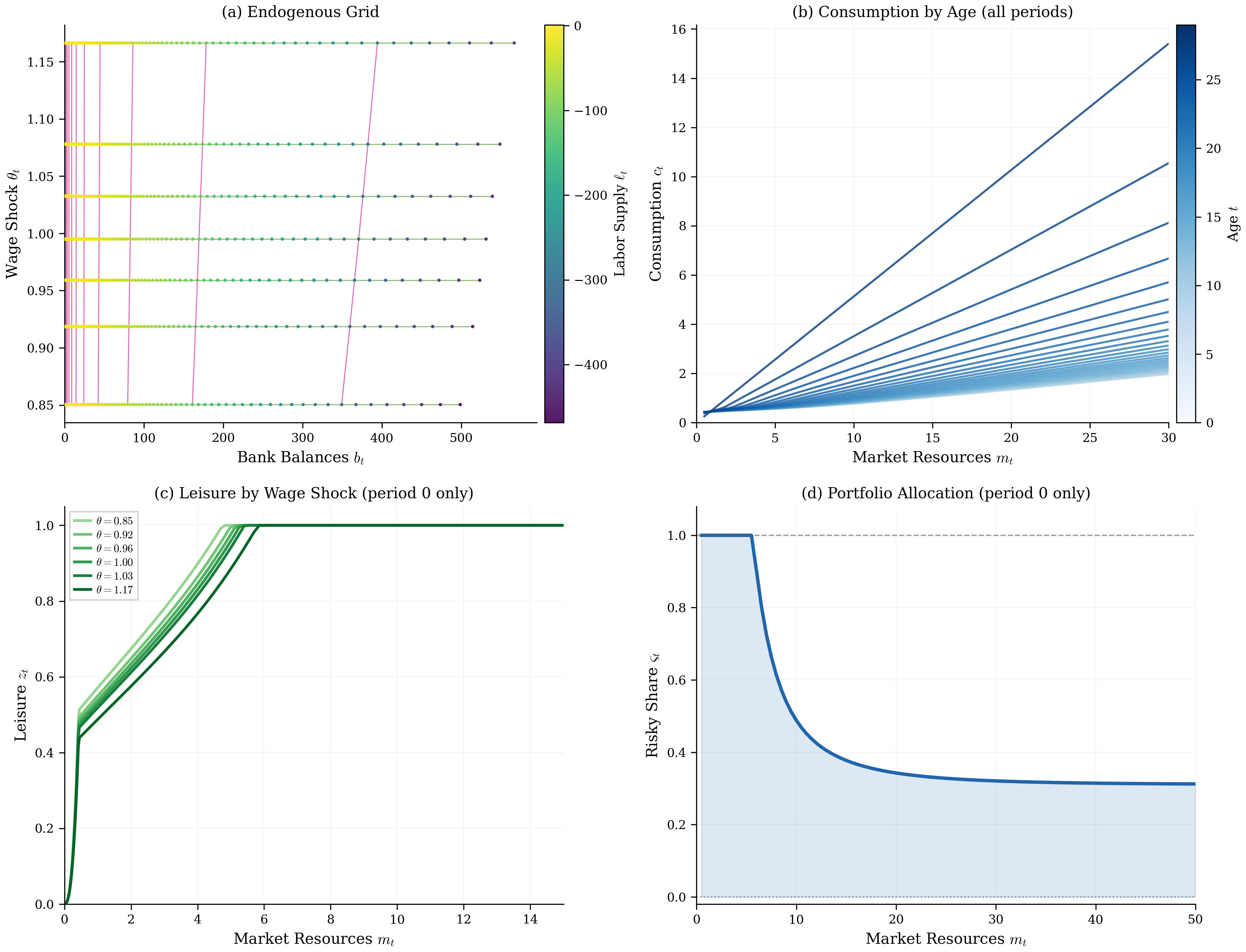
Figure 1:Sequential decomposition produces well-behaved policy functions for the labor-portfolio model (, parameters in footnote).[10] Panel (a) shows the curvilinear endogenous grid from the labor-leisure stage at , colored by optimal labor supply; the grid’s shape is the direct output of EGM inversion, not a post-processing step. Panels (b), (c), and (d) confirm that the three-stage EGM recovers smooth, monotone policy functions. Panel (b) shows that the marginal propensity to consume is higher at low wealth and declines as precautionary savings motives weaken, consistent with buffer-stock theory. Panel (c) shows that lower wages induce more leisure at , since the opportunity cost of not working falls. Panel (d) shows the risky portfolio share at : wealthier households bear more equity risk, a pattern that would be difficult to obtain from a joint three-dimensional optimization without the sequential decomposition.
Figure 1 shows the full solution: panel (a) displays the curvilinear endogenous grid colored by labor supply, panels (b-d) show the consumption, leisure, and portfolio policy functions. The labor-portfolio example demonstrates EGM’s core principle: decompose economically simultaneous decisions into computationally sequential stages, composing EGM inversions without optimization. Sequential decomposition exploited separability in utility (leisure) and transitions (portfolio returns). The labor-leisure stage used EGM inversion; the portfolio stage required convex optimization. Each stage required at most one post-decision state variable, keeping dimensionality manageable. The resulting curvilinear grid from the labor-leisure inversion requires specialized interpolation, addressed in Section 4. Retirement planning with multiple accounts requires tracking several state variables simultaneously across stages, presenting a more demanding test of the method’s applicability.
3The in Higher Dimensions
The labor-portfolio problem in Section 2 features at most one post-decision state variable per stage, keeping dimensionality manageable. Problems where multiple state variables persist across stages present a more demanding test: two state variables must be tracked simultaneously through the EGM inversion. Health investment, durable goods choices, and human capital accumulation all exhibit this structure. The health investment model requires the risk-aversion coefficient for technical reasons detailed below; it serves to illustrate interpolation properties of curvilinear EGM grids rather than realistic calibration. The labor-portfolio model of Section 2 imposes no such restriction. The health investment problem demonstrates that EGM extends to such settings, though the interpolation challenge intensifies: endogenous grids become curvilinear, requiring specialized interpolation methods.
3.1A health investment model
For a demonstration of multivariate EGM, we turn to a consumption-saving model with health investment adapted from White (2015), which itself builds on Ludwig & Schön (2018). This model tests EGM more severely than the labor-portfolio example: two continuous state variables (wealth and health) persist across EGM stages, generating genuinely two-dimensional curvilinear grids. White (2015) designed this model specifically to demonstrate curvilinear interpolation for EGM, so comparing ENGINE against it on the same problem provides a direct test of interpolation methods. In this model, the agent makes decisions about consumption and health investment, subject to wage rate uncertainty, health depreciation risk, and mortality risk that depends on health status.
Each period , the agent observes their market resources and health capital . They choose consumption and health investment to maximize lifetime utility, where denotes the beginning of the planning horizon and denotes the terminal period. Consumption yields CRRA utility, while health investment produces additional health capital through a concave production function. Health capital serves two purposes: it reduces mortality risk and increases labor income through higher productivity.
The recursive problem is:
where the utility function and health production function are:
The notation is as follows: denotes post-investment health capital, is end-of-period assets, is the survival probability (with the maximum death probability applying when health is zero, i.e., ), is the stochastic health depreciation rate, is the stochastic wage rate, and is labor income. The health production scale factor and the health production elasticity determine diminishing returns to health investment. The terminal condition is , so the agent in the final period consumes all remaining resources. The agent trades off current consumption utility against the survival probability , which depends on health through : higher health investment raises and thereby increases the weight placed on future value.[11]
This model requires so that utility is non-negative for all , and that there is positive probability of zero wage (). These restrictions ensure that the first-order conditions are necessary and sufficient to characterize the solution. The restriction implies low risk aversion (below log utility), which limits the model to less risk-averse agents than standard calibrations; the health model serves to illustrate the interpolation properties of curvilinear EGM grids rather than to represent empirically plausible household behavior. The labor-portfolio model of Section 2 imposes no such restriction and uses . As a limiting case, when the health production elasticity (linear production), the marginal product becomes constant, so the EGM inversion at the health investment stage yields a unique solution independent of the state variables, and the problem collapses to a standard consumption-savings problem with an exogenous health process.[12]
3.2Sequential EGM solution
EGM decomposes a problem with multiple controls into a sequence of subproblems, each handling a single control variable. This problem splits into three stages: a health investment stage, a consumption stage, and a post-decision stage that handles expectations. Using the stage superscript convention from Section 2, is the value at the first decision stage (health investment). For the post-decision stage, we use rather than (the notation of Section 2) to emphasize that it represents a post-decision value function (capturing expectations over future shocks) rather than a decision stage. This notation follows Powell (2011) where denotes the post-decision state value.[13] Since all value functions in this section have multiple arguments, we write partial derivatives as superscripts () rather than the prime notation of Section 2; the Appendix uses subscript notation () for second-order terms.
The post-decision stage represents the value of end-of-period states before the realization of next period’s shocks:
where , , and . Conceptualizing this subproblem as a separate stage allows the function to be constructed once and used in prior optimization problems without repeated expectation calculations.[14]
After making their health investment decision, the agent has liquid wealth and post-investment health . The consumption problem is:
Post-investment health passes through this stage unaffected because it enters the continuation value but is not changed by the consumption decision. For each fixed value of , this is a standard one-dimensional consumption-saving problem that can be solved via EGM.[15]
At the beginning of the period, the agent has market resources and health capital . The health investment problem is:
This stage has no direct utility payoff, but the agent’s choice of health investment affects both their liquid wealth (through the budget) and their post-investment health (through the production function). The differentiable and invertible health production function enables an EGM step. The constraint is handled by the Inada condition : the marginal product of health investment grows without bound near zero, so interior solutions obtain whenever the marginal value of health is positive and the agent has resources to invest.[16]
The consumption EGM
The consumption stage applies the same EGM inversion as Section 2, now with health passing through as a parameter. On an exogenous grid of post-decision states , the first-order condition inverts to
The endogenous liquid wealth grid is , and the envelope conditions provide the marginal values needed by the health investment stage:
The health investment stage uses EGM with a differentiable transition. The problem in compact form is:
The first-order condition with respect to is:
Rearranging the first-order condition yields:
Since is invertible, optimal health investment follows:[17]
The transition equations then recover the endogenous pre-decision states:
The envelope conditions provide:[18]
Starting from a regular rectilinear grid of , the health investment EGM step produces a curvilinear endogenous grid of . Figure 2 illustrates this transformation.
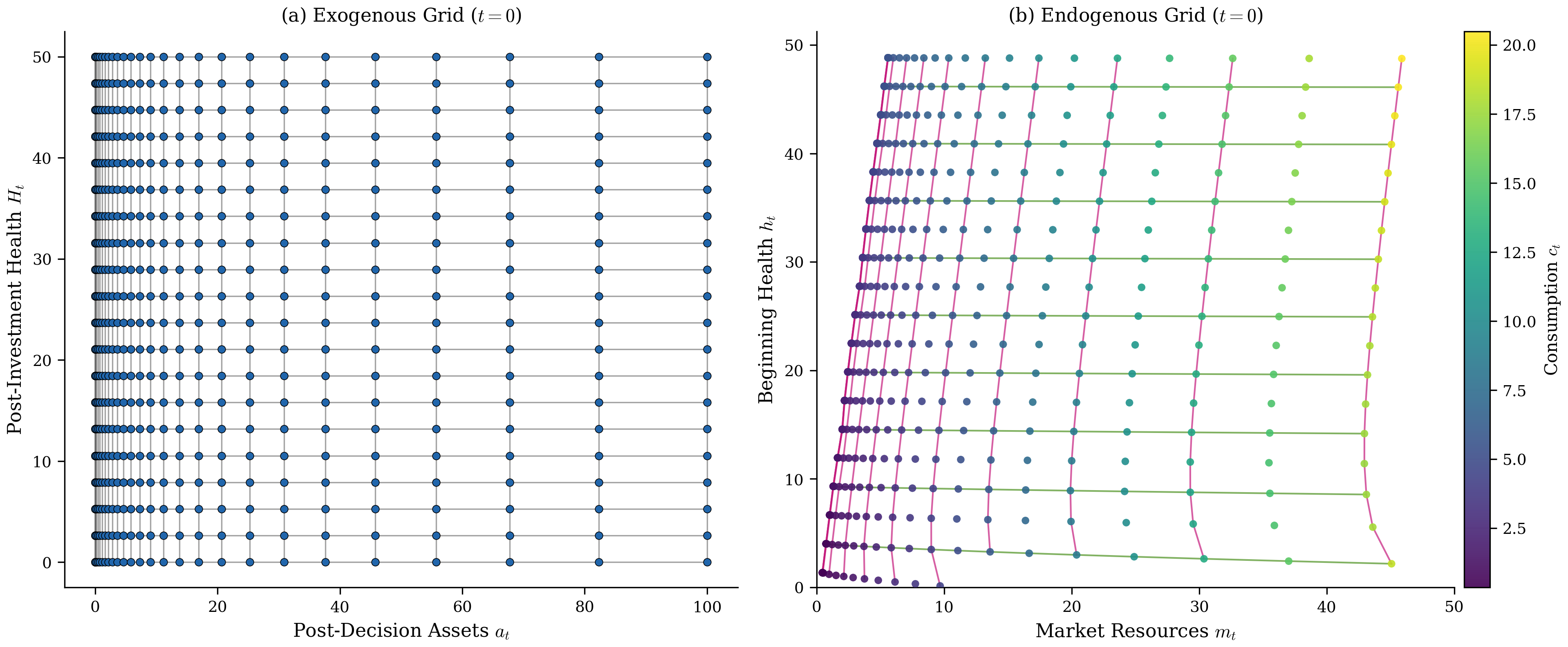
Figure 2:EGM grid transformation for the health investment model at (the first period of economic life). Panel (a) shows the regular exogenous grid of post-decision assets and post-investment health . Panel (b) shows the curvilinear endogenous grid of market resources and beginning-of-period health , with points colored by optimal consumption. The endogenous grid preserves the topological ordering of the exogenous grid despite substantial warping near the constraint boundary, confirming that ENGINE’s index-based interpolation remains valid.[19]
Despite this warping, the endogenous grid maintains the topological structure of the exogenous grid: neighboring points in the grid map to neighboring points in the grid. This property enables efficient interpolation, as discussed in Section 4.
4Multivariate Interpolation on Curvilinear Grids
EGM’s efficiency comes from working on exogenous grids where calculations are straightforward, then using the inverted Euler equation to recover endogenous state variables. But this efficiency creates a problem. The resulting endogenous grid is curvilinear rather than rectilinear, and standard multilinear interpolation, which assumes each dimension varies independently, cannot handle it. What interpolation methods can respect the actual geometry of these grids while exploiting the topological structure that persists despite geometric distortion?
This section presents ENGINE (ENdogenous Grid INterpolation and Extrapolation), which relies on the index structure that endogenous grids inherit from exogenous grids despite geometric warping. ENGINE reduces multidimensional interpolation to a sequence of one-dimensional interpolations along these inherited indices, using the fact that row remains row after warping and neighbors remain neighbors, even when geometric regularity (uniform spacing, rectilinear alignment) is lost.
Consider a curvilinear grid indexed by and , where each “row” (fixed ) contains points. Standard curvilinear interpolation locates the containing quadrilateral cell via sector-walking, then solves for normalized coordinates within that cell (a quadratic equation in 2D, Newton iteration in higher dimensions). ENGINE sidesteps both operations by reframing the problem: instead of asking “which cell contains this point?”, ENGINE asks “where does a vertical line at intersect each row?” For each of the rows, this is a one-dimensional interpolation problem: find where falls among the -coordinates in that row, then interpolate the -coordinate to produce an intermediate point. A final 1D interpolation across these intermediate points yields the answer. The approach works because EGM preserves index structure: point in the exogenous grid maps to a geometrically warped but topologically consistent location in the endogenous grid, so that row remains row and neighbors remain neighbors.
4.1Regularity conditions
The interpolation challenge arises because first-order conditions induce nonlinear mappings from exogenous to endogenous grids. Highly nonlinear or non-monotonic Euler equations can distort grid structure beyond the regular spacing assumed by standard methods. Binding constraints compound the problem by creating kinks in policy functions, introducing additional irregularity.
The pure consumption-savings problem illustrates the basic phenomenon. An exogenous grid of post-decision liquid assets maps through the inverted Euler equation to an endogenous grid of market resources with different spacing; the nonlinearity of marginal utility ensures this mapping is non-uniform. In one dimension, that is no obstacle: non-uniform linear interpolation handles the distortion.
Higher-dimensional problems inherit this warping in each dimension simultaneously, potentially destroying the regular structure assumed by standard multilinear interpolation. The degree of structural preservation determines the appropriate interpolation method. Figure 2 in the previous section illustrates this transformation for the health investment model.
Previous approaches to this problem include Delaunay triangulation Ludwig & Schön, 2018 and curvilinear interpolation White, 2015. Delaunay triangulation constructs a mesh of simplices over the scattered points and performs barycentric interpolation within each simplex. While general and robust, triangulation is computationally expensive, often requiring for construction alone, and must be recomputed when grids change during iterative solution procedures. The curvilinear method takes advantage of the grid structure to map irregular quadrilateral sectors to the unit square for bilinear interpolation; sector location uses a visibility walk algorithm, while coordinate calculation in 2D employs a closed-form quadratic solution (3D and higher require Newton iteration).
ENGINE requires structural conditions on the endogenous grid, but these conditions are not additional assumptions: they follow from the same economic structure that makes EGM applicable. Theorem 2 below proves that any grid produced by an EGM inversion automatically satisfies ENGINE’s requirements, provided the underlying value function is strictly concave and smooth. This applies to standard EGM Carroll, 2006, nested EGM Druedahl, 2021, and the EGM of this paper alike. However, discrete choices pose a problem: when optimal policies jump discontinuously between discrete alternatives, the resulting grids violate monotonicity (IPM) and ENGINE does not apply. Such problems require upper envelope techniques as in G2EGM or DCEGM. The Endogenous Grid Method works when Euler equations are invertible, value functions are strictly concave, and both are twice continuously differentiable. These properties generate well-behaved endogenous grids automatically. A grid satisfying these conditions is homeomorphic to the rectangular index grid: the EGM mapping is a continuous bijection with continuous inverse from index space to physical space.[20]
The conditions separate into two categories: geometric regularity (ensuring a well-defined grid) and algorithmic efficiency (ensuring ENGINE operates efficiently). We state these conditions formally, then prove that grids satisfying them support ENGINE interpolation, and finally show that EGM-generated grids satisfy these conditions automatically.
Nonlinear EGM mappings can distort cells severely enough to invert them. The fold-free condition, the classical validity condition from structured mesh generation Knupp, 1999, ensures each cell maintains proper orientation.
Fold-free ensures local cell validity, but ENGINE also requires that bracketing along rows and columns be well-defined. IPM ensures coordinates increase monotonically along each index direction.
Together, fold-free and IPM ensure the grid mapping is a homeomorphism, guaranteeing interpolation correctness. The final condition, IPO, ensures efficiency: it bounds how fast bracketing indices change across rows, enabling ENGINE to use binary search with bounded search ranges.
When , adjacent rows’ brackets differ by at most one; when , IPO imposes no constraint and ENGINE degenerates to linear search along each row, yielding per query. ENGINE is built around IPO: binary search on rows bounds the search range for at each probe by .
The IPO constant relates to the Lipschitz constant of the EGM mapping. To see this, consider how the bracketing index changes across rows. The EGM mapping transforms exogenous grid points to endogenous coordinates. If this mapping has Lipschitz constant , then for row spacing . For a fixed query , the bracket can therefore shift by at most indices when moving from row to , where is the column spacing. Thus . Strict concavity of the value function bounds (the second derivative controls how fast optimal policies change), so for smooth EGM problems, is typically small.[23]
In practice, can be estimated empirically after solving by computing over a dense set of test points. For the models in this paper, on all grids tested, and empirical query times scale as rather than the worst-case .[24]
With the regularity conditions defined, we now establish their implications. Fold-free and IPM together guarantee that any query point has exactly one location in the grid, so interpolation is well-defined (Theorem 1).
The homeomorphism ensures correctness, but we also need efficiency. The geometric conditions connect to concrete algorithmic guarantees (Corollary 1): IPO bounds how fast brackets change, enabling ENGINE to locate cells without exhaustive search.
The preceding results establish what conditions enable ENGINE. The practical question is whether these conditions impose additional restrictions on practitioners. Standard EGM assumptions (strict concavity, smoothness, monotone marginal utility) imply ENGINE’s conditions automatically (Theorem 2): no additional restrictions arise.
The health investment model of Section 3 illustrates these results: consumption and health investment policies are monotonic (IPM), policy functions vary smoothly (IPO), and the EGM mapping is locally invertible (fold-free). Violations of these conditions typically signal either numerical issues or economic features requiring special treatment.
Occasionally binding constraints, such as borrowing limits, merit explicit discussion. These constraints introduce kinks in policy functions but preserve monotonicity, satisfying IPM, IPO, and fold-free. EGM handles such constraints naturally: the exogenous grid defines the unconstrained (interior) region, and the constrained region is constructed by prepending a point at the constraint boundary (e.g., at for a liquidity constraint). The kink occurs where the policy transitions from corner to interior solution, but on either side of this boundary the policy remains monotonic in wealth. Grid cells straddling the kink may exhibit elevated locally, but ENGINE handles this gracefully by widening the search range. Discrete choices, by contrast, create discontinuities that violate these conditions.
4.2The ENGINE algorithm
ENGINE exploits the index correspondence between endogenous and exogenous grids: each point in the endogenous grid corresponds to indices from the exogenous grid . This structure enables efficient cell location and interpolation without explicit geometric constructions.
There exists a homeomorphism between the curvilinear grid in physical space and the rectilinear grid in index space. Figure 3 illustrates this correspondence: the warped grid on the left maps bijectively and continuously to the regular index grid on the right, with the inverse also continuous, preserving neighborhood relationships. ENGINE works in index space where bracketing is efficient, then inverts the homeomorphism to recover physical coordinates.
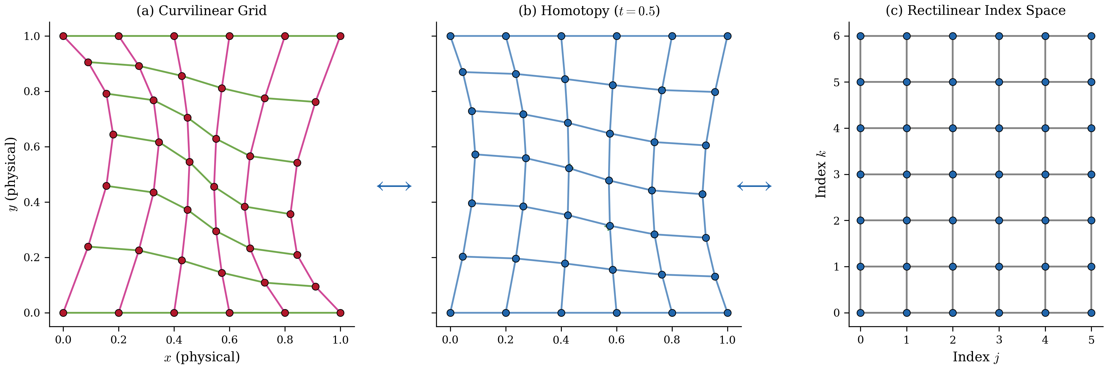
Figure 3:The homeomorphism from physical to index space preserves cell topology despite substantial geometric warping (left: curvilinear physical grid; right: rectilinear index grid). This structure is what makes ENGINE possible: because neighbors remain neighbors after warping, binary search in index space locates the correct cell without geometric operations, reducing cell location from sector-walking to binary search.
The full algorithm is provided in the Appendix. Figure 4 illustrates this process: the vertical line at intersects each -slice of the curvilinear grid, with Pass 1 finding the intermediate -coordinates at these intersections. Pass 2 then interpolates across these intermediate values to produce the final result.
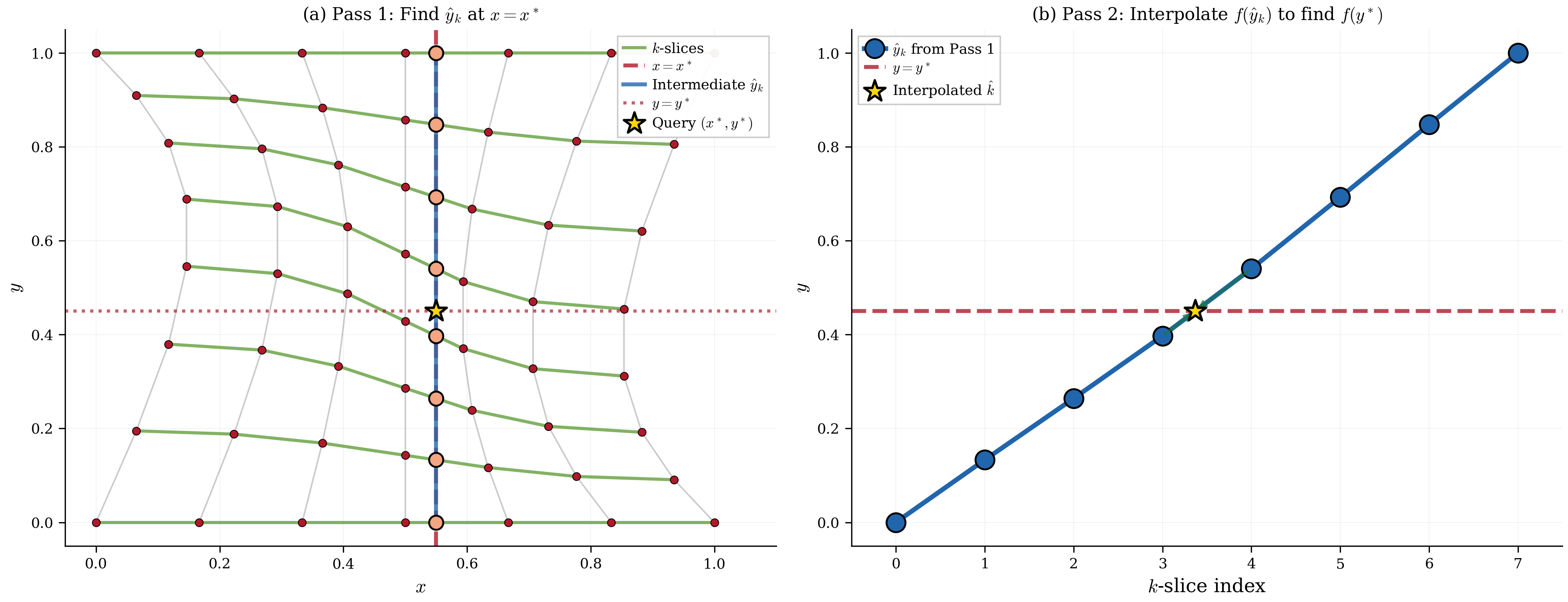
Figure 4:ENGINE reduces 2D interpolation to sequential 1D operations. Pass 1 (panel a): the vertical line at intersects each -slice at intermediate coordinates (circles), each requiring only a 1D bracket search. Pass 2 (panel b): a single 1D interpolation across the intermediate points yields the final value at the query point (star). No cell search, coordinate inversion, or preprocessing is required.
The choice of dimension order (rows versus columns) can affect accuracy when grid warping is highly anisotropic. For the health investment problem, interpolating first along the liquid wealth dimension (which varies more smoothly) and then along the health dimension typically yields better results.
ENGINE sidesteps the cell search and coordinate inversion required by curvilinear methods, requiring only sequential 1D interpolations. The tradeoff is that ENGINE requires IPM and IPO in addition to fold-free, but for EGM-generated grids these conditions hold automatically.
For sorted query points, an additional optimization applies: given sorted queries and sorted grid coordinates , a “walking pointer” bracket index only advances (never backtracks) as queries are processed in order. Finding the enclosing interval for query requires checking whether ; if so, interpolation occurs within ; otherwise, advances until the condition holds. This reduces per-query complexity from to when queries are monotonically ordered, as occurs with meshgrid evaluation.
For a query point , the interpolated value is:
where and are the intermediate coordinates and values from Pass 1.
The preceding theorems established that ENGINE is well-defined and efficient on EGM-generated grids. Decomposing 2D interpolation into sequential 1D operations does not sacrifice accuracy: the method achieves the same second-order convergence as standard bilinear interpolation (Proposition 1).
With accuracy established, Proposition 2 formalizes the complexity analysis. IPO bounds how fast brackets change across rows, enabling ENGINE to reuse bracket information from previous probes rather than searching from scratch.
The method offers several computational advantages: natural parallelization across query points (each query is independent), efficient memory access patterns from sequential array traversal, and no preprocessing or Newton iteration in any dimension.[27]
Extension to higher dimensions
ENGINE extends naturally to dimensions via sequential passes. For a problem with indices :
Pass 1 interpolates along the direction for each combination of .
Pass 2 interpolates along the direction using the results from Pass 1.
Continue until Pass produces the final interpolated value.
The total complexity for a single query scales as when using the naive approach that evaluates all intermediate slices. Binary search optimizations analogous to the 2D case can reduce this, but the gains depend on higher-dimensional analogues of IPO that bound bracket displacement across multiple index dimensions simultaneously.[28]
4.3Comparison with alternative methods
The three approaches to multi-dimensional EGM interpolation differ in their algorithmic strategy for handling curvilinear endogenous grids:
| Method | Setup | Query Cost | Interpolation | Grid Requirements |
|---|---|---|---|---|
| ENGINE (this paper) | Sequential linear | Fold-free + IPM + IPO() | ||
| Curvilinear White, 2015 | Bilinear | Fold-free only | ||
| Delaunay Ludwig & Schön, 2018 | Piecewise linear | None |
ENGINE achieves per query, which is asymptotically faster than curvilinear’s sector-walking. For smooth EGM problems with small IPO constant , empirical performance approaches . Benchmarks show 2-3x speedups depending on grid size, with larger gains at larger grids.
Figure 5 illustrates how these three methods partition the state space. Bilinear interpolation identifies the containing quadrilateral cell and computes normalized coordinates within it. Delaunay triangulation constructs a mesh of triangles and uses barycentric coordinates. ENGINE processes the grid slice-by-slice, interpolating along indexed rows before combining intermediate results.
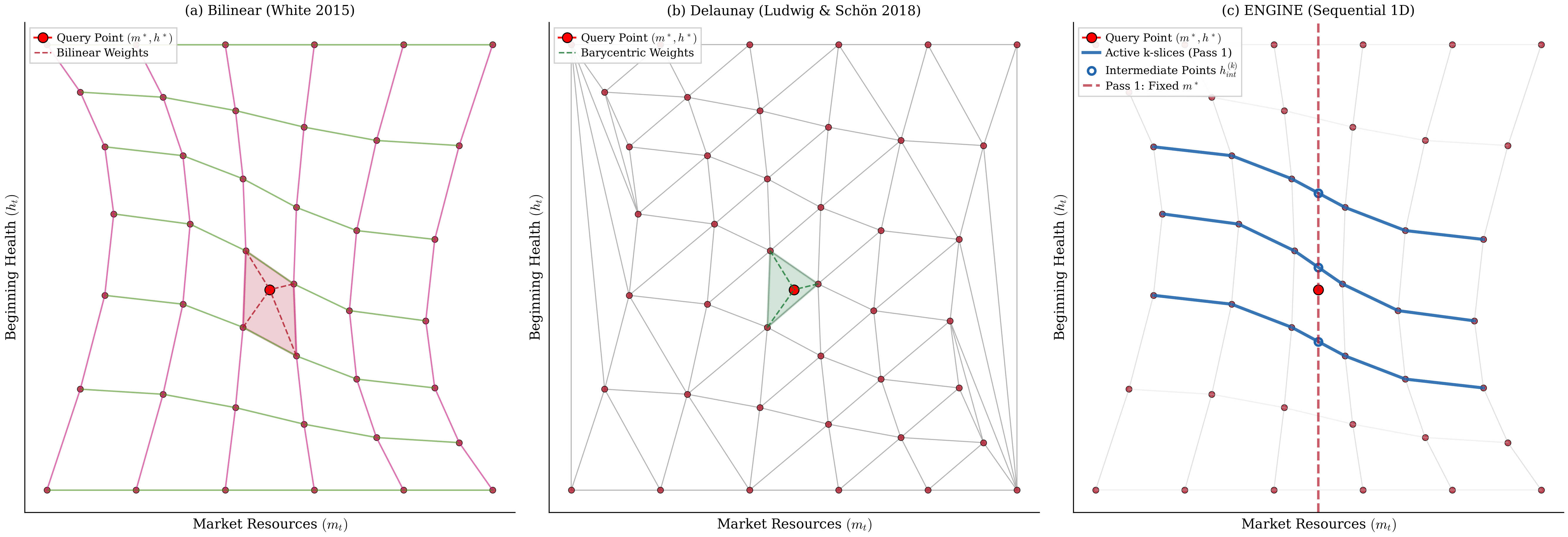
Figure 5:All three methods correctly partition the state space, but ENGINE’s slice-based structure is cheaper to traverse. Bilinear interpolation searches for the containing quadrilateral (panel a), Delaunay triangulation constructs simplices from scratch (panel b), and ENGINE interpolates sequentially along indexed -slices (highlighted curves) before combining intermediate points (circles) to reach the query point (star) in panel (c). The index structure inherited from the exogenous grid makes panel (c) reducible to binary search, while panels (a) and (b) require geometric operations without that structure.
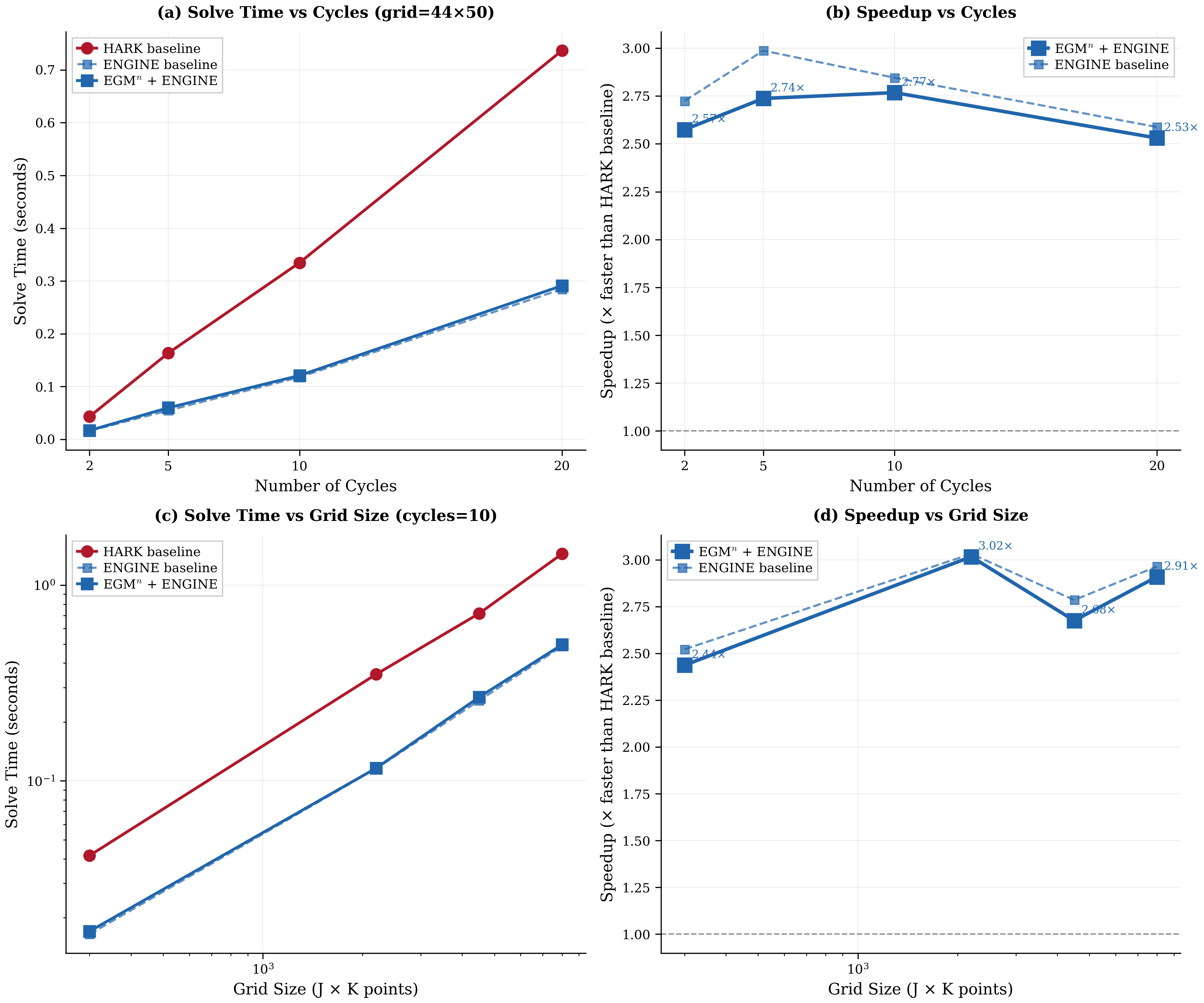
Figure 6:Performance comparison on the health investment model. Panels (a) and (b) show solve time and speedup versus the number of backward induction cycles at fixed grid size (). Panels (c) and (d) show solve time and speedup versus grid size at fixed cycle count (10). EGM + ENGINE achieves 2-3x speedups over the curvilinear interpolation baseline of White (2015) depending on grid size.
Figure 6 compares ENGINE against the curvilinear interpolation of White (2015) across both time horizon (cycles) and grid resolution.[29] The benchmarks use the health investment model of Section 3 with , providing a direct comparison on the same model class for which curvilinear interpolation was developed. As noted in Section 3, the restriction is specific to this health formulation; the benchmarks illustrate interpolation performance on curvilinear grids rather than an economically calibrated model. Speedups scale with grid size as the complexity advantage materializes; accuracy matches standard bilinear interpolation per Proposition 1.
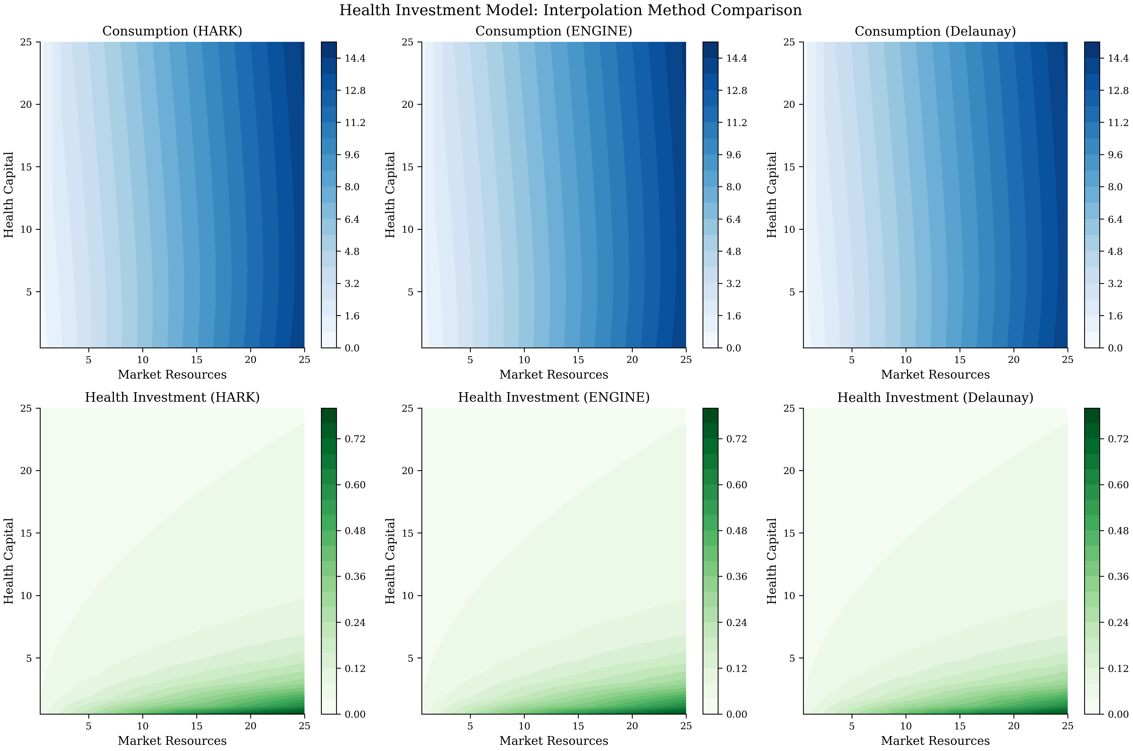
Figure 7:Policy functions for the health investment model computed using different interpolation methods. The top row shows the consumption function and the bottom row shows the health investment function . All three interpolation methods (curvilinear interpolation of White (2015), ENGINE, and Delaunay triangulation) produce visually indistinguishable policy surfaces: maximum pointwise differences are below 10-4 at all grid points tested.
For the health investment model, the dominant cost components in the backward induction loop are: expectation calculations (computing marginal value functions on the exogenous grid via quadrature), interpolation (evaluating value and marginal value functions on the curvilinear endogenous grid), and EGM inversion (recovering endogenous states from first-order conditions). At typical grid sizes (), interpolation accounts for roughly 40-50% of solve time, expectations for 30-40%, and EGM inversion for the remainder. ENGINE’s speedup therefore translates most directly into the interpolation component, explaining why total solve-time speedups (2-3x) are smaller than the asymptotic complexity ratio might suggest.
ENGINE provides efficient interpolation when grids satisfy fold-free, IPM, and IPO. By Theorem 2, any EGM inversion under standard conditions (strict concavity, smoothness) produces such grids automatically. The next section addresses a separate question: when can a multidecision problem be decomposed into EGM stages? The separability and invertibility conditions there determine when EGM applies, completing the practical toolkit for applying these methods to new problems.
5Conditions for Sequential Decomposition
When does EGM apply? The labor-portfolio problem (Section 2) and health investment problem (Section 3) illustrated two key structures: separable utility functions and invertible transitions. This section formalizes these requirements and provides practical guidance for decomposing new problems. The examples demonstrated specific instances; we now characterize the general conditions that make sequential decomposition with EGM inversion possible.
5.1Splitting the problem into subproblems
Decomposition begins by counting independent control variables. A problem with control variables typically decomposes into subproblems. One must take care not to double-count: the consumption-savings choice () represents one decision, not two. Similarly, labor-leisure is a single choice despite involving two variables.
Each control variable requires an enabling structure that permits EGM inversion. Two mathematical structures suffice: separable, differentiable, and invertible utility functions (as in the leisure utility of Section 2); or differentiable and invertible transition functions (as in the health production function of Section 3). Match each control variable to its enabling structure. The labor-portfolio example features additive utility separability: leisure utility enables the labor-leisure EGM step, consumption utility enables the consumption-savings EGM step. When no structure applies (as in the portfolio choice stage), standard optimization is required.
The ordering of subproblems should shed state variables early. Poor sequencing propagates unnecessary state variables through later stages. In the consumption-leisure-portfolio problem, placing labor-leisure first resolves the wage rate before the consumption stage, keeping that subproblem one-dimensional. Choosing consumption first would force the labor decision to track both bank balances and wages, doubling its dimensionality.[30]
5.2Formal conditions
We now abstract from specific models to general conditions. The notation shifts to uppercase calligraphic functions (, , , , ) for generic value, continuation, utility, transition, and shock functions, with generic state variables , , in place of the model-specific variables: consumption , assets , and cash-on-hand of preceding sections.
Consider a utility function of the form
where is the vector of control variables, is the -th control variable, and is the vector of all control variables except the -th one. This utility function is separable in the control variable corresponding to index .
We collect the discounted continuation value into a single function:
Substituting, the problem reduces to:
When post-decision states are multidimensional, with components for and transition functions mapping controls to each component (here superscripts on and index components, not derivatives), the first-order condition (FOC) with respect to control (assuming an interior solution) becomes
The requirement for (separability in the transition) is sufficient to solve for independently. This condition ensures that control affects only the -th post-decision state, decoupling the FOC from other transition equations. When transition separability fails, the first-order conditions couple across stages, requiring simultaneous solution of all controls — exactly the computational burden that sequential EGM is designed to avoid.[31]
Under transition separability, the first-order condition for stage simplifies to:
Each stage’s optimality condition depends only on its own control and the continuation value, not on controls chosen at other stages.
Separable utility
Once the problem is split into subproblems, the Endogenous Grid Method applies to each applicable subproblem while iterating backwards from the terminal period. The EGM step applies when there is a separable, differentiable and invertible utility function in the subproblem or when there is a differentiable and invertible transition in the subproblem.
To see when the method fails, consider non-separable CES preferences . The first-order condition (FOC) for consumption involves leisure: . Inverting for requires knowing , and the symmetric condition for requires knowing . The FOCs are coupled, so neither can be solved in isolation by EGM inversion. Such problems require joint root-finding (NEGM) or upper envelope techniques (G2EGM).
Consider a generic subproblem with a differentiable and invertible utility function:
where is the continuation value. For an interior solution, the first-order condition is
When corner solutions occur (e.g., at constraint boundaries), the unconstrained optimum from inverting the first-order condition must be projected onto the feasible set, as demonstrated in Section 2 for the leisure choice.
The question is when this first-order condition can be inverted to yield the optimal control directly. Proposition 3 gives the standard case: separable utility with a transition linear in the control, which covers most consumption-savings applications.
The linearity assumption is satisfied by standard budget constraints appearing in consumption-savings models. For example, implies , so . Similarly, the labor income constraint has , which varies with the wage shock but is constant with respect to the control . Linearity in the control allows the first-order condition to be inverted analytically, which is the computational step that replaces root-finding. State-dependent coefficients (like ) are permissible provided they are known when solving the subproblem.
Using an exogenous grid of the post-decision state , the optimal decision rule follows at each point on the grid. This inversion replaces a numerical root-find with a single function evaluation, the core speed advantage of EGM. The monotonicity requirement ensures that the mapping from the post-decision state to the control is well-defined, while concavity guarantees uniqueness of the optimal decision at each grid point.
Proposition 3 covers the standard case where utility is separable. But some subproblems have no within-period utility at all, only transitions affecting multiple post-decision states. Health investment in Section 3 is such a case: there is no immediate utility from health spending, only effects on future health and wealth. Proposition 4 shows that EGM still applies when transitions are invertible, even without separable utility. Consider a problem with two endogenous state variables and two post-decision states:
where the continuation value is
The first-order condition becomes
Additive separability in both transitions allows the derivative with respect to to not depend on the state variables or , which have not yet been recovered when solving the first-order condition on the exogenous grid of post-decision states. Once is obtained from the inversion, the pre-decision states follow via and . The formulation where one state variable enters linearly (e.g., with and ) is a common special case.
This additive separability defines what Iskhakov (2015) calls “triangular” structure in transitions. The triangular property enables the multidimensional EGM to proceed without root-finding: when the FOC system has triangular form, each control can be recovered sequentially by substitution rather than by solving a coupled nonlinear system. Their approach solves problems where the entire multidimensional structure is triangular, enabling simultaneous solution of all choices with applications to wealth accumulation, health capital, and portfolio problems. Together, the two propositions characterize the practical scope of EGM: sequential EGM applies whenever each subproblem satisfies either separable utility (Proposition 1) or invertible transitions (Proposition 2), and the decomposition ordering can be chosen to satisfy these conditions stage by stage.
6Conclusion
EGM applies when the problem satisfies a few structural conditions. Each condition has a natural economic interpretation: separability reflects that the marginal utility of one choice does not depend on the level of another; triangularity reflects that each decision’s consequences flow forward in time without looping back.
First, the utility function must be additively separable across controls, or the transition functions linking controls to post-decision states must be differentiable and invertible. Second, choices must be continuous with smooth resulting policy functions; discrete choices require G2EGM or the Discrete-Continuous EGM (DCEGM). Third, the first-order conditions for different controls must decouple; coupled FOCs require NEGM or G2EGM.
When EGM applies, ENGINE handles interpolation on the resulting curvilinear grids with no preprocessing and natural parallelization. The ordering of subproblems should minimize the information set passed forward: the labor-portfolio example sequences (leisure-labor, consumption-savings, portfolio) so each stage sheds state variables before the next. When subproblems are independent, as with consumption and health investment affecting different state dimensions, ordering is immaterial.
The two examples confirm that economically simultaneous decisions need not be computationally joint: the labor-portfolio problem eliminates optimization at two of three stages, and the health model avoids root-finding entirely. When separable structure permits decomposition, most stages admit EGM inversion, passing efficiency gains forward through the stage sequence. ENGINE (ENdogenous Grid INterpolation and Extrapolation) addresses the interpolation challenge by exploiting the index correspondence inherited from exogenous grids, achieving 2-3x speedups over existing curvilinear interpolation.
A multistage problem can mix stages satisfying separable utility (Proposition 3) with stages satisfying triangular transitions (Proposition 4), and even include stages solved by standard optimization, expanding applicability beyond problems that require joint inversion of coupled first-order conditions across all decisions. The same smoothness conditions that enable EGM inversion also determine ENGINE’s efficiency: strict concavity bounds the Lipschitz constant of the EGM mapping, which in turn bounds the IPO constant that controls interpolation complexity. Problems with smooth value functions typically have small , enabling ENGINE’s complexity (with empirical performance approaching for smooth problems).
Relative to NEGM Druedahl, 2021, which nests root-finding or optimization within EGM loops, EGM avoids all numerical solution steps when its structural assumptions hold; and relative to triangular EGM Iskhakov, 2015, which requires triangularity of the entire FOC system, EGM requires only sequential invertibility at each stage, permitting mixed structures. G2EGM Druedahl & Jørgensen, 2017 handles discrete choices and non-convexities through upper envelope techniques, a domain where EGM does not apply. ENGINE complements this by providing efficient interpolation with no preprocessing, simple implementation, and efficient memory access patterns.
Limitations
Problems with non-separable utility (e.g., consumption-leisure complementarity where FOCs are coupled) or correlated transitions require alternative methods such as G2EGM or NEGM. ENGINE’s regularity conditions (fold-free, IPM, IPO) follow automatically from EGM’s standard regularity assumptions (strict concavity, smoothness), so they impose no additional burden on applicable problems. However, problems with discrete choices or severe non-convexities violate EGM’s assumptions and hence ENGINE’s conditions, requiring alternative methods; occasionally binding constraints typically preserve monotonicity and remain tractable. ENGINE’s multilinear interpolation faces a curse of dimensionality: each interpolation requires cell vertices, making problems with state variables computationally challenging regardless of the interpolation method.
Several extensions merit future investigation. Combining EGM stages with G2EGM’s upper envelope techniques could handle problems where some decisions are separable while others involve discrete choices. Adaptive grid refinement could concentrate computational effort in regions where policy functions exhibit rapid variation. The sequential structure also facilitates parallelization: independent EGM inversions across grid points can be distributed across processors with minimal coordination cost.
Applications that become newly tractable include high-frequency portfolio rebalancing with transaction costs and multiple asset classes, multiperiod health insurance choices with endogenous health states and moral hazard, and durable goods decisions with both extensive and intensive margins. The efficiency gains from avoiding triangulation setup costs and exploiting efficient memory access patterns make structural estimation via simulated method of moments or maximum likelihood more practical, particularly when the model must be solved thousands of times during optimization. Some models are simply waiting for a faster solver. Models of consumption response to fiscal stimulus Kaplan & Violante, 2014, wealth accumulation over the life cycle Cagetti, 2003, and household balance sheet dynamics Fagereng et al., 2021 all feature multiple interacting decisions that can benefit from sequential decomposition when their structure permits.
The EGM and ENGINE algorithms are available as open-source software, allowing researchers to apply sequential decomposition and index-based interpolation to their own multidimensional lifecycle models.[34]
6.1Declaration of generative AI and AI-assisted technologies in the manuscript preparation process
During the preparation of this work the author used Claude (Anthropic) in order to edit and proofread the manuscript and to assist with coding. After using this tool, the author reviewed and edited the content as needed and takes full responsibility for the content of the published article.
Acknowledgments
I would like to thank Chris Carroll, Matthew White, and Fedor Iskhakov for their helpful comments and suggestions. The remaining errors are my own. This paper was awarded the Outstanding Graduate Student Paper Award at the 29th International Conference on Computing in Economics and Finance (CEF 2023, Nice, France). Presentations at the Johns Hopkins University Macro Brownbag (2024), the International Association for Applied Econometrics annual conference (2024, Thessaloniki, Greece), and the University of Texas at Austin MA in Economics Program 10-Year Reunion Celebration (2024) improved the exposition and applications. The author received support through the Econ-ARK project funded by a grant from the Alfred P. Sloan Foundation during the development of this work. All figures and other numerical results were produced using the Econ-ARK/HARK toolkit Carroll et al., 2018.
In companion work, Lujan (2026) extends EGM to Epstein-Zin preferences via a power transformation, complementing the multi-decision approach developed here.
See Maliar & Maliar (2014) for a thorough survey of numerical methods for such problems.
An alternative formulation expresses preferences in terms of disutility of labor as , which gives and for . This formulation does not support a balanced growth path because labor disutility is not homogeneous of degree in permanent income.
Following Carroll (2009). Since both utility components are homogeneous of degree in , the level utility can be written as , and dividing the Bellman equation by yields the stationary normalized recursive formulation.
Specifically: (i) utility and value functions are twice continuously differentiable in the interior of the constraint set; (ii) the Inada conditions and hold, ensuring interior solutions away from zero consumption; and (iii) constraint sets are convex with non-empty interior. These conditions ensure first-order conditions are necessary for optimality at interior solutions. Strict concavity of the utility and value functions further ensures sufficiency: any point satisfying the FOC is a global maximum.
An alternative formulation defines where embeds the expectation. Both marginal value functions and can then be computed in one expectation step, avoiding redundant integration.
With the functional form , the Inada condition ensures the lower bound never binds for finite wages and marginal values. At the upper bound , the agent chooses full leisure when , which occurs for sufficiently low wages or high wealth.
The labor-leisure problem could be solved using simpler interpolation methods since the grid warping occurs along only one dimension. Curvilinear Grid Interpolation is used here to demonstrate the sequential decomposition that is the essence of EGM and to illustrate CGI in a transparent setting before encountering the two-dimensional curvilinear grids of Section 3.
Parameters follow HARK defaults: , , . Risky returns are lognormally distributed with mean 1.08 and standard deviation 0.18. Wage shocks are lognormally distributed with standard deviation 0.1. Labor-specific parameters are and .
The concave production function with exhibits diminishing returns to health investment. The marginal product is strictly decreasing and satisfies the Inada conditions and , ensuring interior solutions for health investment when resources permit.
With , utility is negative and the product would reward mortality. The restriction mirrors White (2015) and is specific to this health formulation, not to EGM generally. Models with mortality risk and can use a bequest motive or utility differences; see De Nardi (2004).
Computing the post-decision value function separately improves computational efficiency by avoiding redundant expectation calculations. The marginal value functions and can be computed once on an exogenous grid and interpolated as needed by earlier stages. Note that includes both the survival probability benefit of health (through ) and the continuation value benefit (through next period’s health).
Unlike the consumption stage, which exploits separable utility, this stage exploits a differentiable and invertible transition function. The health production function plays a role analogous to the matching function in pension deposit problems: both provide the mathematical structure needed for EGM inversion without requiring separable utility.
Strict monotonicity of ensures the inverse is well-defined. For the power function, since , confirming strict monotonicity. The inverse is .
The envelope conditions follow from the fact that both and enter the value function only through the post-decision states and . The first-order condition ensures that the marginal effects of adjusting cancel out, leaving only the direct effects of the state variables on continuation value.
The figure uses , , , health production exponent , health depreciation rate , wage rate with mean 0.1 and standard deviation 0.1, and a two-period model (, so the agent lives periods ).
IPM and IPO are new terms introduced here. The standard characterization of a valid curvilinear coordinate system is that the grid mapping is a homeomorphism.
The discrete Jacobian equals twice the signed area of the triangle formed by vertices , , and . Equivalently, it is the cross product of edge vectors and . Positive means these vectors form a right-handed (counterclockwise) pair; negative indicates the cell has folded (inverted orientation); zero indicates degeneracy. The four-corner condition is standard in the structured mesh generation literature Knupp, 1999 and is stronger than requiring positivity only at the lower-left corner. For EGM-generated grids, Theorem 2 establishes that the continuous Jacobian throughout each cell, automatically satisfying the four-corner condition.
When constraint regions produce constant policies along a grid dimension (e.g., zero consumption at the borrowing constraint), adjacent grid points may have identical coordinates. The implementation handles this by (1) skipping zero-width intervals during bracket search, (2) using one-sided limits at degeneracy boundaries, and (3) treating constant-policy regions as a single effective grid point. These cases are rare for well-designed grids that concentrate resolution in economically active regions.
Economically, becomes large when policy functions change rapidly relative to grid spacing, which occurs near occasionally binding constraints or when the value function has high curvature (strong precautionary motives, tight borrowing limits). In such regions, the EGM mapping stretches or compresses the grid non-uniformly. Standard practice in computational economics uses log-spaced or double-log-spaced grids that concentrate resolution where policies vary most, which keeps moderate. Highly anisotropic grids (very different spacing in different dimensions) can also inflate ; balanced grid design mitigates this.
The implementation uses a configurable curvature bound (default ) that controls the search margin: when probing row after previously probing row , the -bracket search range is bounded by indices around the previous bracket.
When conditions are partially violated, ENGINE degrades gracefully. If IPM fails but fold-free holds, linear search replaces binary search, yielding . Only when fold-free fails (grid folds over itself) must one resort to unstructured methods.
Here denotes the maximum cell diameter. The rate for piecewise linear interpolation is standard Boor, 2001. On curvilinear grids the bound holds when the grid mapping Jacobian is bounded away from zero and infinity, which fold-free and IPM ensure. Composing two interpolations preserves this order because intermediate values have bounded variation when the original function is smooth.
The implementation uses NumPy Harris et al., 2020 with Numba Lam et al., 2015 just-in-time compilation within the Econ-ARK HARK toolkit Carroll et al., 2018. The 2-3x speedups reflect both algorithmic gains (reduced complexity from to per query) and cache-friendly sequential access patterns. When multiple functions share the same endogenous grid, the cell-location work from Pass 1 is reused across all functions.
ENGINE’s sequential approach avoids the exponential complexity of triangulation-based methods in higher dimensions. For a three-dimensional problem with grid points, Delaunay triangulation requires construction time. The naive ENGINE approach requires per query; with appropriate regularity conditions, binary search can reduce this toward , though the conditions ensuring this are more complex than the 2D case.
Both ENGINE and the baseline use the HARK toolkit’s Carroll et al., 2018 Numba-compiled interpolation routines, so the comparison is between equivalently compiled codebases.
To see this concretely, the consumption subproblem would become two-dimensional: subject to , requiring interpolation on a grid instead of just . The labor-leisure subproblem would then have the additional constraint: subject to and . The poor ordering forces us to carry the wage state through both stages, doubling the dimensionality of the first stage.
Separability is sufficient but not strictly necessary. Alternative structures may also permit independent solution: for example, a triangular system where depends on but not on allows sequential substitution, solving for first, then given , and so on. However, separability is the most common and practically verifiable condition.
Strict monotonicity of the marginal utility ensures that the inverse function is well-defined and single-valued. This condition is satisfied by standard utility functions like CRRA utility where is strictly decreasing in consumption.
Strict monotonicity of ensures the inverse is well-defined. In the health investment example, the production function satisfies this property with strictly decreasing for .
The algorithms are implemented in the
ConsSequentialEGMSolverandCurvilinearInterpclasses within the Econ-ARK HARK toolkit Carroll et al., 2018.
- Carroll, C., Kaufman, A., Kazil, J., Palmer, N., & White, M. (2018). The econ-ARK and HARK: Open source tools for computational economics. In F. Akici, D. Lippa, D. Niederhut, & M. Pacer (Eds.), Proceedings of the Python in Science Conference (pp. 25–30). SciPy. 10.25080/majora-4af1f417-004
- Aiyagari, S. R. (1994). Uninsured Idiosyncratic Risk and Aggregate Saving. The Quarterly Journal of Economics, 109(3), 659–684. 10.2307/2118417
- Huggett, M. (1993). The Risk-Free Rate in Heterogeneous-Agent Incomplete-Insurance Economies. Journal of Economic Dynamics and Control, 17(5–6), 953–969. 10.1016/0165-1889(93)90024-M
- Krueger, D., Mitman, K., & Perri, F. (2016). Macroeconomics and household heterogeneity. In Handbook of Macroeconomics (Vol. 2, pp. 843–921). Elsevier. 10.1016/bs.hesmac.2016.04.003
- Iskhakov, F. (2015). Multidimensional endogenous gridpoint method: Solving triangular dynamic stochastic optimization problems without root-finding operations. Economics Letters, 135, 72–76. 10.1016/j.econlet.2015.07.033
- Druedahl, J., & Jørgensen, T. H. (2017). A general endogenous grid method for multi-dimensional models with non-convexities and constraints. Journal of Economic Dynamics and Control, 74, 87–107. 10.1016/j.jedc.2016.11.005
- Carroll, C. D. (2006). The method of endogenous gridpoints for solving dynamic stochastic optimization problems. Economics Letters, 91(3), 312–320. 10.1016/j.econlet.2005.09.013
- Barillas, F., & Fernández-Villaverde, J. (2007). A generalization of the endogenous grid method. Journal of Economic Dynamics and Control, 31(8), 2698–2712. 10.1016/j.jedc.2006.08.005
- Fella, G. (2014). A generalized endogenous grid method for non-smooth and non-concave problems. Review of Economic Dynamics, 17(2), 329–344. 10.1016/j.red.2013.07.001
- Hintermaier, T., & Koeniger, W. (2010). The method of endogenous gridpoints with occasionally binding constraints among endogenous variables. Journal of Economic Dynamics and Control, 34(10), 2074–2088. 10.1016/j.jedc.2010.05.002
- Iskhakov, F., Jørgensen, T. H., Rust, J., & Schjerning, B. (2017). The endogenous grid method for discrete-continuous dynamic choice models with (or without) taste shocks. Quantitative Economics, 8(2), 317–365. 10.3982/QE643
- Clausen, A., & Strub, C. (2020). Reverse calculus and nested optimization. Journal of Economic Theory, 187(105019), 105019. 10.1016/j.jet.2020.105019
- Hallengreen, A., Jørgensen, T. H., & Olesen, A. M. (2024). The Endogenous Grid Method without Analytical Inverse Marginal Utility (Working Paper No. 24–11). University of Copenhagen, Center for Economic Behavior. 10.2139/ssrn.4830404
- Jørgensen, T. H. (2013). Structural estimation of continuous choice models: Evaluating the EGM and MPEC. Economics Letters, 119(3), 287–290. 10.1016/j.econlet.2013.02.027
- White, M. N. (2015). The method of endogenous gridpoints in theory and practice. Journal of Economic Dynamics and Control, 60, 26–41. 10.1016/j.jedc.2015.08.001