Labor-Portfolio Choice with EGM^n - EGMⁿ: The Sequential Endogenous Grid Method

This notebook applies the Sequential Endogenous Grid Method (EGM $^n$ ) to a consumption-saving model with both endogenous labor supply and portfolio choice. This is the primary example from the paper, where the agent simultaneously chooses consumption $c_t$ , labor supply $\ell_t$ (equivalently, leisure $z_t = 1 - \ell_t$ ), and portfolio allocation $\varsigma_t$ (share in risky asset).

import sys
sys.path.append("../")

import matplotlib.pyplot as plt
import numpy as np
from ConsLaborSeparableModel import LaborPortfolioConsumerType
from HARK.utilities import plot_funcs

1The Model¶

The agent’s problem combines labor-leisure choice with portfolio allocation:

v_t(m_t, \theta_t) = \max_{c_t, z_t, \varsigma_t} u(c_t) + h(z_t) + \beta \mathbb{E}_t[\Gamma_{t+1}^{1-\rho} v_{t+1}(m_{t+1}, \theta_{t+1})]

(1)

subject to:

Market resources: $m_t = b_t + \theta_t \cdot (1 - z_t)$
Saving: $a_t = m_t - c_t$
Portfolio return: $R^p_{t+1} = R^f + (R^e_{t+1} - R^f) \varsigma_t$
Next period: $m_{t+1} = a_t R^p_{t+1} / \Gamma_{t+1} + \theta_{t+1}$

def plot_3d_func(func, lims_x, lims_y, n=100, label_x="x", label_y="y", label_z="z"):
    """Helper function to plot 3D policy surfaces."""
    xmin, xmax = lims_x
    ymin, ymax = lims_y
    xgrid = np.linspace(xmin, xmax, n)
    ygrid = np.linspace(ymin, ymax, n)
    xMat, yMat = np.meshgrid(xgrid, ygrid, indexing="ij")
    zMat = func(xMat, yMat)
    
    ax = plt.axes(projection="3d")
    ax.plot_surface(xMat, yMat, zMat, cmap="viridis", alpha=0.8)
    ax.set_xlabel(label_x)
    ax.set_ylabel(label_y)
    ax.set_zlabel(label_z)
    plt.show()

# Create agent with 10 life-cycle periods
agent = LaborPortfolioConsumerType()
agent.cycles = 10

2Solving the Model¶

The solver proceeds backward through three stages per period:

Portfolio stage: given end-of-period assets $a_t$ , find optimal risky share $\varsigma_t$
Consumption stage: given liquid wealth $\ell_t$ , find optimal consumption $c_t$
Labor stage: given bank balances $b_t$ and wage $\theta_t$ , find optimal labor $1 - z_t$

agent.solve()
print(f"Solved {len(agent.solution)} periods")

Solved 11 periods

3Examining the Solution Structure¶

Each period’s solution contains the policy functions from all three stages:

# Access the solution for the first period
sol = agent.solution[0]

# The three stages
share_func = sol.portfolio_stage.share_func    # Portfolio choice
c_func = sol.consumption_stage.c_func          # Consumption
labor_func = sol.labor_stage.labor_func        # Labor supply
leisure_func = sol.labor_stage.leisure_func    # Leisure (1 - labor)

Portfolio Choice¶

The optimal risky share as a function of end-of-period assets:

plot_funcs(share_func, 0, 100)
plt.xlabel("End-of-Period Assets $a_t$")
plt.ylabel("Risky Share $\\varsigma_t$")
plt.title("Portfolio Allocation Policy")
plt.show()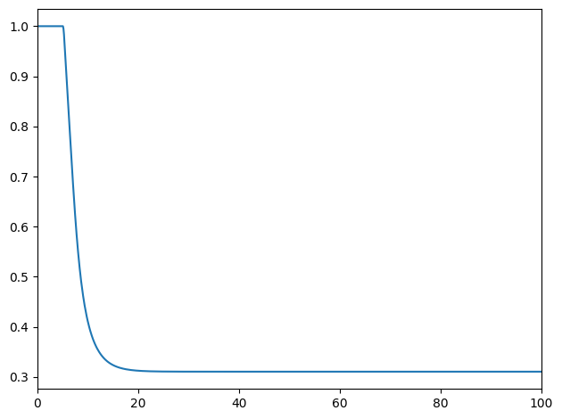

Consumption Function¶

plot_funcs(c_func, 0, 100)
plt.xlabel("Market Resources $m_t$")
plt.ylabel("Consumption $c_t$")
plt.title("Consumption Policy")
plt.show()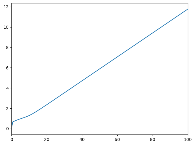

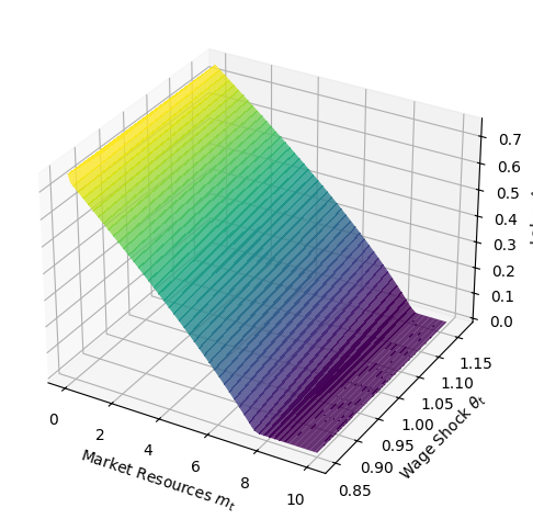
Labor Supply¶

The labor function depends on both market resources and the wage shock:

theta_grid = agent.TranShkGrid
if hasattr(theta_grid, '__len__'):
    theta_min, theta_max = min(theta_grid), max(theta_grid)
else:
    theta_min, theta_max = 0.5, 1.5

plot_3d_func(
    labor_func,
    (0, 10),
    (theta_min, theta_max),
    label_x="Market Resources $m_t$",
    label_y="Wage Shock $\\theta_t$",
    label_z="Labor $\\ell_t$",
)

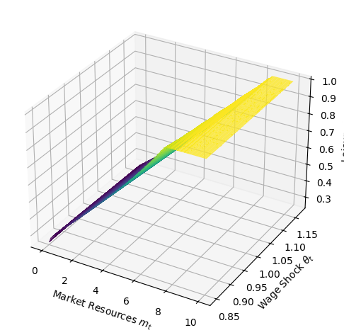
plot_3d_func(
    leisure_func,
    (0, 10),
    (theta_min, theta_max),
    label_x="Market Resources $m_t$",
    label_y="Wage Shock $\\theta_t$",
    label_z="Leisure $z_t$",
)

Consumption Cross-Sections¶

plot_funcs(agent.solution[0].consumption_stage.c_func, 0, 10)
plt.xlabel("Market Resources $m_t$")
plt.ylabel("Consumption $c_t$")
plt.title("Consumption Policy at $t=0$")
plt.show()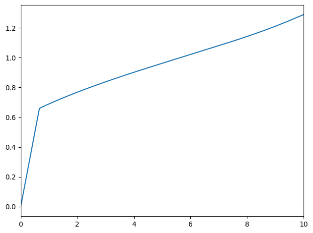

4Computational Approach¶

Joint optimization over $(c_t, z_t, \varsigma_t)$ would typically require a 3D grid search or nonlinear root-finding. EGM $^n$ instead solves each stage by inverting first-order conditions, producing curvilinear endogenous grids that ENGINE interpolates. The computational cost scales linearly with grid size rather than exponentially. See the paper for the mathematical derivation and the ENGINE interpolation algorithm.