ENGINE: Interpolation on Curvilinear Grids - EGMⁿ: The Sequential Endogenous Grid Method

ENGINE: Interpolation on Curvilinear Grids

This notebook documents ENGINE (ENdogenous Grid INterpolation and Extrapolation), an interpolation method for curvilinear grids that arise from the Endogenous Grid Method.

import sys
sys.path.insert(0, "..")

import matplotlib.pyplot as plt
import numpy as np
from mpl_toolkits.mplot3d import Axes3D
import time

from engine2d import Engine2DInterp, warmup_jit
from HARK.interpolation import Curvilinear2DInterp
from scipy.interpolate import LinearNDInterpolator

1The Curvilinear Grid Problem¶

Assume we have a set of points indexed by $(j, k)$ in 2D space for which we have corresponding function values: $f(x_{jk}, y_{jk}) = z_{jk}$ .

In practice, we are interested in cases where computing $z$ is expensive (e.g., solving a dynamic programming problem), so we want to interpolate rather than recompute. The challenge is that these $(x_{jk}, y_{jk})$ points are not evenly spaced and do not form a rectilinear grid.

For illustration, we use $f(x,y) = (xy)^{1/4}$ :

# Create a simple curvilinear grid (hand-crafted example)
points = np.array(
    [[[1, 7], [3, 8], [5, 9]], 
     [[2, 2], [4, 4], [6, 6]], 
     [[7, 1], [8, 3], [9, 5]]]
).T
values = np.power(points[0] * points[1], 1/4)

fig, ax = plt.subplots(figsize=(8, 6))
sc = ax.scatter(points[0], points[1], c=values, cmap="viridis", s=100, edgecolor="black")
plt.colorbar(sc, label="Function value $f(x,y)$")
ax.set_xlabel("$x$")
ax.set_ylabel("$y$")
ax.set_title("Curvilinear Grid Points")
ax.grid(True, alpha=0.3)
plt.show()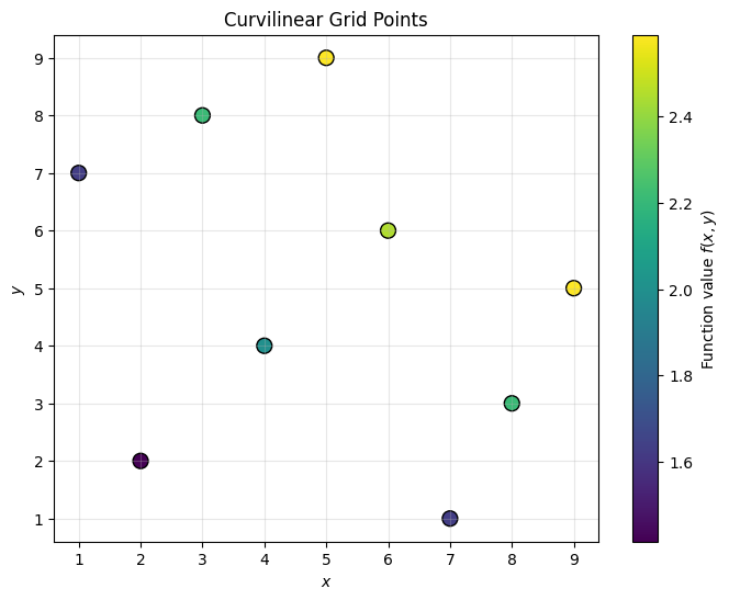

2The Topological Structure¶

Although these points don’t form a rectangular grid in physical space, they have a crucial property: topological regularity. Points that are neighbors in the index space $(j, k)$ remain neighbors in the physical space $(x, y)$ .

# Show the grid structure: curvilinear vs index space
fig, axes = plt.subplots(1, 2, figsize=(12, 5))

# Left: Curvilinear grid in physical space
ax = axes[0]
ax.scatter(points[0], points[1], c="blue", s=80, zorder=5)
for j in range(3):
    ax.plot(points[0, j, :], points[1, j, :], "g-", lw=2, alpha=0.7, 
            label="$j$-slices" if j == 0 else "")
for k in range(3):
    ax.plot(points[0, :, k], points[1, :, k], "r-", lw=2, alpha=0.7,
            label="$k$-slices" if k == 0 else "")
ax.set_xlabel("$x$")
ax.set_ylabel("$y$")
ax.set_title("(a) Curvilinear Grid in Physical Space")
ax.legend()
ax.grid(True, alpha=0.3)

# Right: Regular index space
ax = axes[1]
coord_points = np.mgrid[0:3, 0:3]
ax.scatter(coord_points[0], coord_points[1], c="blue", s=80, zorder=5)
for j in range(3):
    ax.plot(coord_points[0, j, :], coord_points[1, j, :], "g-", lw=2, alpha=0.7)
for k in range(3):
    ax.plot(coord_points[0, :, k], coord_points[1, :, k], "r-", lw=2, alpha=0.7)
ax.set_xlabel("Index $j$")
ax.set_ylabel("Index $k$")
ax.set_title("(b) Regular Index Space")
ax.grid(True, alpha=0.3)

plt.tight_layout()
plt.show()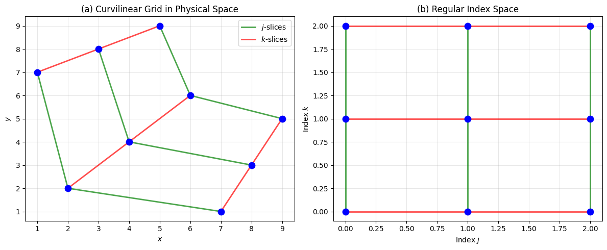

3Visualizing the True Function¶

fig = plt.figure(figsize=(10, 7))
ax = fig.add_subplot(projection="3d")

# True function surface
x = np.linspace(1, 9, 50)
xmat, ymat = np.meshgrid(x, x, indexing="ij")
zmat = np.power(xmat * ymat, 1/4)
ax.plot_surface(xmat, ymat, zmat, alpha=0.4, cmap="viridis")

# Known grid points
ax.scatter(points[0], points[1], values, c="red", s=100, edgecolor="black")

# Projections to floor
ax.scatter(points[0], points[1], np.zeros_like(values), c="blue", alpha=0.3)
for i in range(9):
    ax.plot([points[0].flat[i]]*2, [points[1].flat[i]]*2, 
            [0, values.flat[i]], "--", c="blue", alpha=0.3)

ax.set_xlabel("$x$")
ax.set_ylabel("$y$")
ax.set_zlabel("$f(x,y)$")
ax.set_title("True Function $f(x,y) = (xy)^{1/4}$ with Known Grid Points")
ax.view_init(30, -120)
plt.show()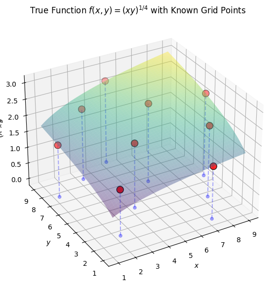

4Alternative Interpolation Methods¶

Before introducing ENGINE, let’s consider the alternatives:

Method 1: Quad/Bilinear Interpolation¶

The “correct” approach would be to:

Find the quadrilateral cell containing the query point
Compute local coordinates $(u, v) \in [0,1]^2$ within the cell
Apply bilinear interpolation

This requires solving a nonlinear system to find $(u, v)$ , which is computationally expensive.

Method 2: Delaunay Triangulation¶

Scipy’s LinearNDInterpolator ignores the grid structure entirely and creates a triangulation. This:

Discards known relationships between points
Requires expensive triangulation (especially for evolving grids)
Cannot easily incorporate derivative information

Method 3: Two-Pass Sequential Interpolation (ENGINE)¶

ENGINE exploits the grid structure via two sequential 1D interpolation passes:

# Visualize the two-pass algorithm
query_x, query_y = 3.0, 5.0

fig, axes = plt.subplots(1, 2, figsize=(14, 5))

# Panel 1: Pass 1 - finding intermediate y-coordinates
ax = axes[0]
ax.scatter(points[0], points[1], c="blue", s=80, zorder=5)
for j in range(3):
    ax.plot(points[0, j, :], points[1, j, :], "g-", lw=2, alpha=0.7)
for k in range(3):
    ax.plot(points[0, :, k], points[1, :, k], "r-", lw=2, alpha=0.7)

ax.axvline(x=query_x, color="cyan", linestyle="--", lw=2.5, label="$x = x^*$")
ax.scatter([query_x]*2, [3.0, 8.0], c="orange", s=150, marker="o", 
           edgecolor="black", lw=2, zorder=8, label=r"Intermediate $\hat{y}_k$")
ax.scatter(query_x, query_y, c="magenta", s=200, marker="*", zorder=10)

ax.set_xlabel("$x$")
ax.set_ylabel("$y$")
ax.set_title(r"Pass 1: Find $\hat{y}_k$ for each $k$-slice at $x = x^*$")
ax.legend(loc="upper right")
ax.grid(True, alpha=0.3)

# Panel 2: Pass 2 - interpolating to find final value
ax = axes[1]
k_indices = np.array([0, 1, 2])
y_intermediate = np.array([3.0, 5.5, 8.0])  # Approximate intermediate values

ax.plot(k_indices, y_intermediate, "o-", color="orange", lw=3, ms=12, 
        mec="black", mew=1.5, label=r"$\hat{y}_k$ from Pass 1")
ax.axhline(y=query_y, color="purple", linestyle="--", lw=2.5, label="$y = y^*$")

# Find interpolated k
k_interp = np.interp(query_y, y_intermediate, k_indices)
ax.scatter(k_interp, query_y, c="magenta", s=200, marker="*", zorder=10,
           label="Interpolated result")

ax.set_xlabel("$k$-slice index")
ax.set_ylabel("$y$")
ax.set_title(r"Pass 2: Interpolate along $\hat{y}_k$ to find $f(x^*, y^*)$")
ax.legend(loc="upper left")
ax.grid(True, alpha=0.3)

plt.tight_layout()
plt.show()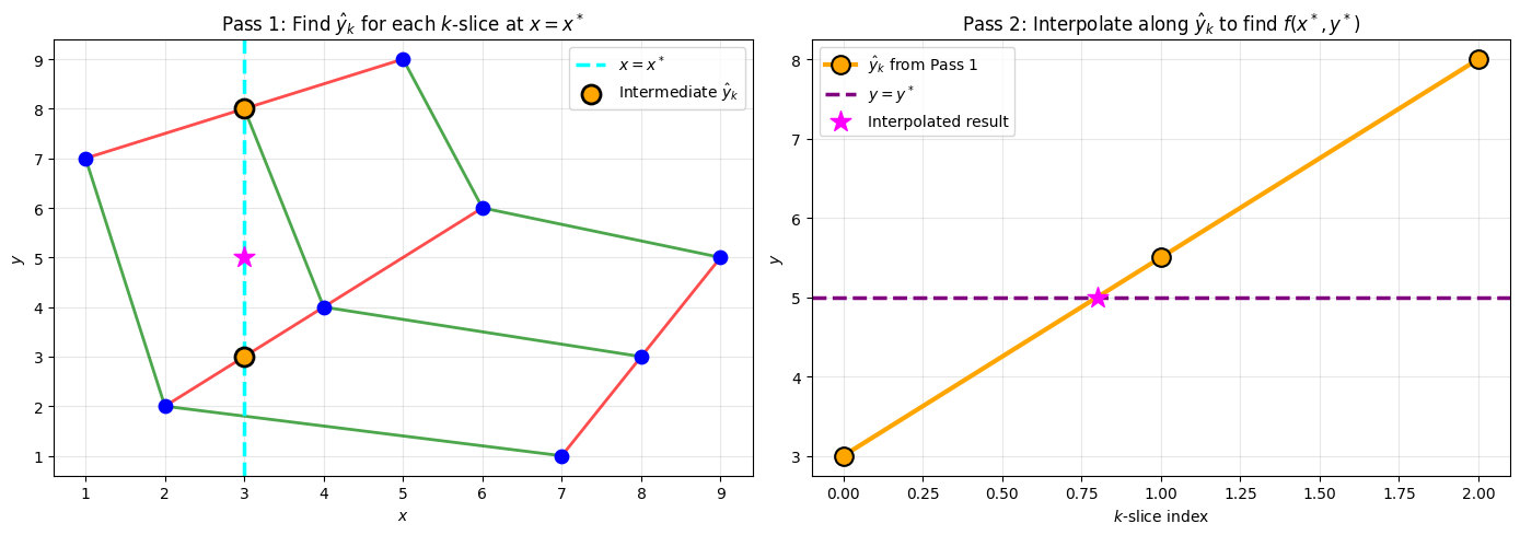

5JIT Warmup for Fair Benchmarks¶

Both ENGINE and HARK’s Curvilinear interpolator use JIT compilation. We must warm them up before timing:

print("Warming up JIT compilation...")
warmup_jit()
print("ENGINE JIT warmup complete!")

Warming up JIT compilation...
ENGINE JIT warmup complete!

6Creating a Realistic Test Grid¶

# Create a larger, more realistic curvilinear grid
np.random.seed(42)
J, K = 15, 18

# Start with a regular grid and apply warping (simulating EGM output)
j_idx = np.arange(J)
k_idx = np.arange(K)
JJ, KK = np.meshgrid(j_idx, k_idx, indexing="ij")

# Apply nonlinear warping
warp_strength = 0.12
x_grid = JJ.astype(float) + warp_strength * np.sin(2 * np.pi * KK / K) * JJ
y_grid = KK.astype(float) + warp_strength * np.cos(2 * np.pi * JJ / J) * KK

# Function values: distance from origin
z_grid = np.sqrt(x_grid**2 + y_grid**2)

print(f"Grid shape: {x_grid.shape} ({J*K} points)")
print(f"x range: [{x_grid.min():.2f}, {x_grid.max():.2f}]")
print(f"y range: [{y_grid.min():.2f}, {y_grid.max():.2f}]")

Grid shape: (15, 18) (270 points)
x range: [0.00, 15.65]
y range: [0.00, 19.04]

# Visualize the warped grid
fig, ax = plt.subplots(figsize=(10, 8))

for k in range(K):
    ax.plot(x_grid[:, k], y_grid[:, k], "g-", lw=0.6, alpha=0.5)
for j in range(J):
    ax.plot(x_grid[j, :], y_grid[j, :], "r-", lw=0.6, alpha=0.5)

sc = ax.scatter(x_grid, y_grid, c=z_grid, cmap="viridis", s=25, 
                edgecolor="black", linewidth=0.3)
plt.colorbar(sc, label="$f(x,y) = \\sqrt{x^2 + y^2}$")

ax.set_xlabel("$x$")
ax.set_ylabel("$y$")
ax.set_title(f"Curvilinear Grid ({J}×{K} = {J*K} points)")
plt.show()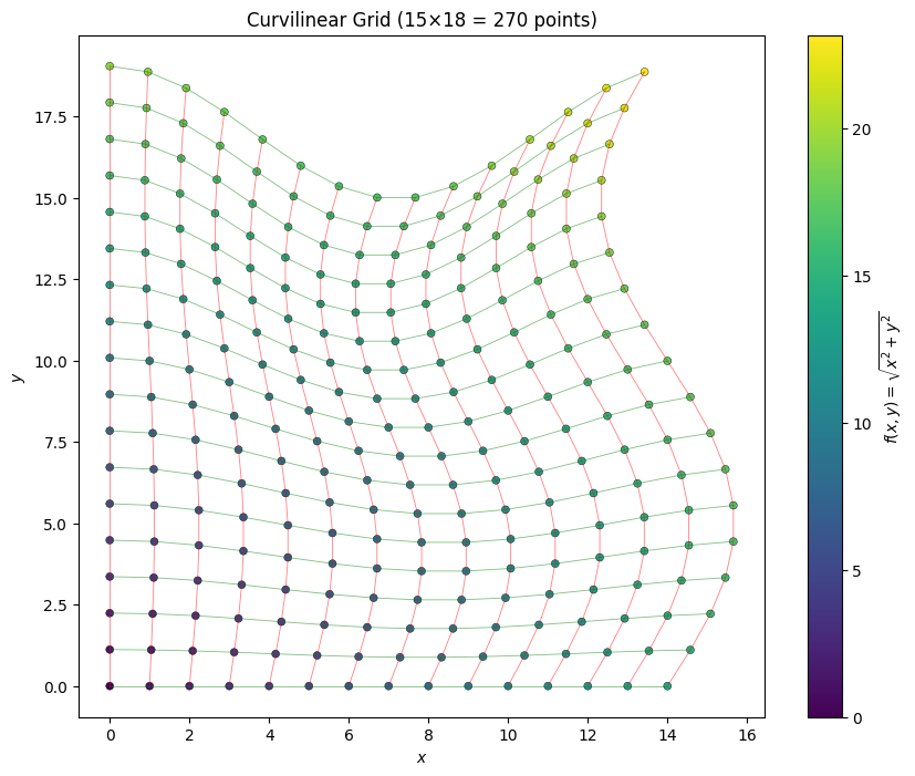

7Creating Interpolators¶

# Create all three interpolators
print("Creating interpolators...")

# ENGINE
engine_interp = Engine2DInterp(z_grid, x_grid, y_grid)
print("  ENGINE interpolator created")

# HARK Curvilinear (sector-walking)
hark_interp = Curvilinear2DInterp(z_grid, x_grid, y_grid)
print("  HARK Curvilinear interpolator created")

# Delaunay (scipy)
delaunay_interp = LinearNDInterpolator(
    np.column_stack([x_grid.ravel(), y_grid.ravel()]), 
    z_grid.ravel()
)
print("  Delaunay interpolator created")

Creating interpolators...
  ENGINE interpolator created

  HARK Curvilinear interpolator created
  Delaunay interpolator created

8Warmup All Interpolators¶

# Generate test query points
x_min, x_max = x_grid.min() + 0.5, x_grid.max() - 0.5
y_min, y_max = y_grid.min() + 0.5, y_grid.max() - 0.5

n_warmup = 100
x_warmup = np.random.uniform(x_min, x_max, n_warmup)
y_warmup = np.random.uniform(y_min, y_max, n_warmup)

# Warmup calls (JIT compilation happens here)
print("Warming up interpolators with test queries...")
_ = engine_interp(x_warmup, y_warmup)
_ = hark_interp(x_warmup, y_warmup)
_ = delaunay_interp(x_warmup, y_warmup)
print("All interpolators warmed up!")

Warming up interpolators with test queries...

All interpolators warmed up!

9Timing Comparison¶

# Fair timing comparison after warmup
n_test = 2000
n_repeats = 50

x_test = np.random.uniform(x_min, x_max, n_test)
y_test = np.random.uniform(y_min, y_max, n_test)

# Time ENGINE
times_engine = []
for _ in range(n_repeats):
    t0 = time.perf_counter()
    _ = engine_interp(x_test, y_test)
    times_engine.append(time.perf_counter() - t0)
engine_time = np.median(times_engine)

# Time HARK Curvilinear
times_hark = []
for _ in range(n_repeats):
    t0 = time.perf_counter()
    _ = hark_interp(x_test, y_test)
    times_hark.append(time.perf_counter() - t0)
hark_time = np.median(times_hark)

# Time Delaunay
times_delaunay = []
for _ in range(n_repeats):
    t0 = time.perf_counter()
    _ = delaunay_interp(x_test, y_test)
    times_delaunay.append(time.perf_counter() - t0)
delaunay_time = np.median(times_delaunay)

print(f"Timing for {n_test} queries (median of {n_repeats} runs):")
print(f"  ENGINE:           {engine_time*1000:.3f} ms")
print(f"  HARK Curvilinear: {hark_time*1000:.3f} ms")
print(f"  Delaunay:         {delaunay_time*1000:.3f} ms")
print(f"\nSpeedups relative to ENGINE:")
print(f"  vs HARK Curvilinear: {hark_time/engine_time:.2f}×")
print(f"  vs Delaunay:         {delaunay_time/engine_time:.2f}×")

Timing for 2000 queries (median of 50 runs):
  ENGINE:           0.407 ms
  HARK Curvilinear: 0.883 ms
  Delaunay:         0.774 ms

Speedups relative to ENGINE:
  vs HARK Curvilinear: 2.17×
  vs Delaunay:         1.90×

# Visualize timing comparison
fig, ax = plt.subplots(figsize=(8, 5))

methods = ["ENGINE", "HARK\nCurvilinear", "Delaunay"]
times = [engine_time*1000, hark_time*1000, delaunay_time*1000]
colors = ["#2ecc71", "#3498db", "#e74c3c"]

bars = ax.bar(methods, times, color=colors, edgecolor="black", linewidth=1.2)

# Add time labels on bars
for bar, t in zip(bars, times):
    ax.text(bar.get_x() + bar.get_width()/2, bar.get_height() + 0.5, 
            f"{t:.2f} ms", ha="center", va="bottom", fontsize=11, fontweight="bold")

ax.set_ylabel("Time (milliseconds)", fontsize=12)
ax.set_title(f"Interpolation Time for {n_test} Queries\n(after JIT warmup)", fontsize=13)
ax.spines["top"].set_visible(False)
ax.spines["right"].set_visible(False)
plt.tight_layout()
plt.show()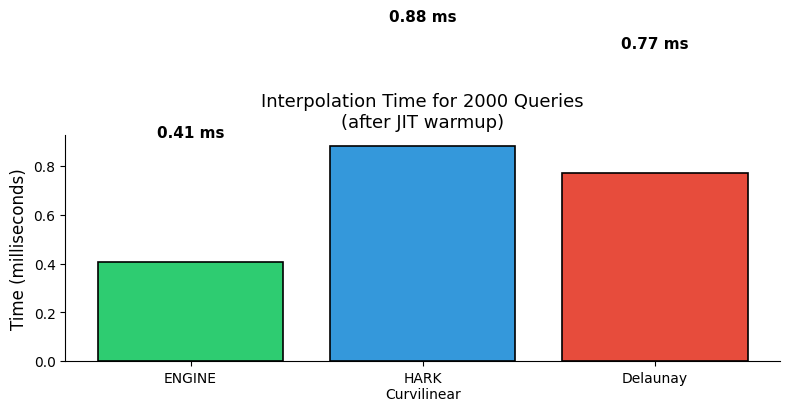

10Accuracy Comparison¶

# Compare accuracy across methods
z_engine = engine_interp(x_test, y_test)
z_hark = hark_interp(x_test, y_test)
z_delaunay = delaunay_interp(x_test, y_test)
z_true = np.sqrt(x_test**2 + y_test**2)

# Handle any NaNs from Delaunay (outside convex hull)
valid_delaunay = ~np.isnan(z_delaunay)

print("Accuracy Comparison:")
print(f"  {'Method':<20} {'Mean Abs Error':<18} {'Max Abs Error':<18} {'Rel Error %'}")
print("-" * 75)
print(f"  {'ENGINE':<20} {np.mean(np.abs(z_engine - z_true)):<18.6f} "
      f"{np.max(np.abs(z_engine - z_true)):<18.6f} "
      f"{np.mean(np.abs(z_engine - z_true)/z_true)*100:.4f}%")
print(f"  {'HARK Curvilinear':<20} {np.mean(np.abs(z_hark - z_true)):<18.6f} "
      f"{np.max(np.abs(z_hark - z_true)):<18.6f} "
      f"{np.mean(np.abs(z_hark - z_true)/z_true)*100:.4f}%")
print(f"  {'Delaunay':<20} {np.nanmean(np.abs(z_delaunay - z_true)):<18.6f} "
      f"{np.nanmax(np.abs(z_delaunay[valid_delaunay] - z_true[valid_delaunay])):<18.6f} "
      f"{np.nanmean(np.abs(z_delaunay - z_true)/z_true)*100:.4f}%")

Accuracy Comparison:
  Method               Mean Abs Error     Max Abs Error      Rel Error %
---------------------------------------------------------------------------
  ENGINE               0.010954           0.148322           0.1411%
  HARK Curvilinear     0.011005           0.172752           0.1455%
  Delaunay             0.038205           0.692465           0.2944%

# Visualize accuracy comparison
fig, axes = plt.subplots(1, 3, figsize=(15, 4))

methods = [
    ("ENGINE", z_engine, "#2ecc71"),
    ("HARK Curvilinear", z_hark, "#3498db"),
    ("Delaunay", z_delaunay, "#e74c3c")
]

for ax, (name, z_pred, color) in zip(axes, methods):
    errors = np.abs(z_pred - z_true)
    mae = np.nanmean(errors)
    
    sc = ax.scatter(z_true, z_pred, c=errors, cmap="Reds", s=15, alpha=0.6)
    ax.plot([z_true.min(), z_true.max()], [z_true.min(), z_true.max()], 
            "k--", lw=2, label="Perfect")
    ax.set_xlabel("True value")
    ax.set_ylabel("Interpolated value")
    ax.set_title(f"{name}\n(MAE: {mae:.5f})")
    plt.colorbar(sc, ax=ax, label="Abs Error")
    ax.legend()

plt.tight_layout()
plt.show()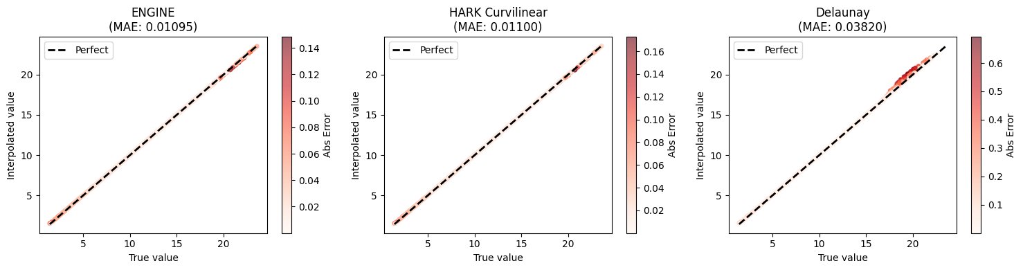

11Why Not Use Scipy’s griddata?¶

# Demonstrate regridding approach (Method 3 from old notebook)
all_coords = np.mgrid[1:int(x_grid.max()):20j, 1:int(y_grid.max()):20j]

fig, ax = plt.subplots(figsize=(8, 6))

# Original curvilinear grid
for k in range(K):
    ax.plot(x_grid[:, k], y_grid[:, k], "g-", lw=0.5, alpha=0.3)
for j in range(J):
    ax.plot(x_grid[j, :], y_grid[j, :], "r-", lw=0.5, alpha=0.3)

# Regular evaluation grid
ax.scatter(all_coords[0], all_coords[1], c="gold", s=30, alpha=0.7, 
           label="Regular evaluation grid", edgecolor="black", linewidth=0.3)
ax.scatter(x_grid, y_grid, c="blue", s=15, alpha=0.6, label="Original curvilinear grid")

ax.set_xlabel("$x$")
ax.set_ylabel("$y$")
ax.set_title("Regridding: Interpolate onto Regular Grid")
ax.legend()
ax.grid(True, alpha=0.2)
plt.show()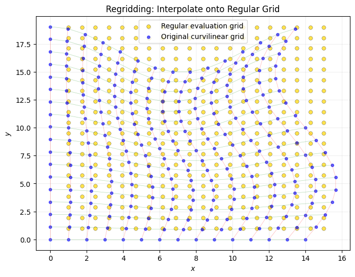

Curvilinear grids arise from EGM by inverting first-order conditions, but the topological regularity (index neighbors remain geometric neighbors) is preserved. ENGINE exploits this structure via two-pass sequential 1D interpolation. See the paper for the full mathematical treatment.