Labor-Leisure Choice with EGM^n

This notebook applies the Sequential Endogenous Grid Method (EGM $^n$ ) to a consumption-saving model with endogenous labor supply. The agent simultaneously chooses consumption $c_t$ and labor supply $\ell_t$ . Rather than solving this as a joint optimization, EGM $^n$ exploits the separable structure to solve each decision sequentially via the Endogenous Grid Method.

import sys
sys.path.append("../")

import matplotlib.pyplot as plt
import numpy as np
from ConsLaborSeparableModel import LaborSeparableConsumerType
from utilities import plot_3d_func
from HARK.utilities import plot_funcs

1The Model¶

Each period, the agent observes bank balances $b_t$ and wage shock $\theta_t$ , then chooses consumption $c_t$ and leisure $z_t = 1 - \ell_t$ . The budget constraint is:

m_t = b_t + \theta_t \cdot \ell_t

(1)

where $m_t$ is market resources available for consumption and saving. The agent’s problem can be written as:

v_t(b_t, \theta_t) = \max_{c_t, z_t} u(c_t) + h(z_t) + \beta \mathbb{E}_t[v_{t+1}(b_{t+1}, \theta_{t+1})]

(2)

# Create an agent with 10 life-cycle periods
agent = LaborSeparableConsumerType(aXtraNestFac=-1, aXtraCount=25, cycles=10)

/mnt/c/Users/alujan/GitHub/alanlujan91/sequential_egm/.venv/lib/python3.12/site-packages/HARK/rewards.py:39: RuntimeWarning: divide by zero encountered in power
  return c ** (1.0 - rho) / (1.0 - rho)

2The Endogenous Grid¶

A key insight of the paper is that EGM produces curvilinear grids. Let’s visualize this by examining the terminal period solution.

# Access the terminal period grids
grids = agent.solution_terminal.terminal_grids

Endogenous Grid in $(b, \theta)$ Space¶

The first-order conditions define optimal labor as a function of the exogenous grid. When we invert to find the endogenous states, the regular grid becomes warped:

fig, axes = plt.subplots(1, 2, figsize=(12, 5))

# Panel 1: Endogenous grid (bank balances vs wage shock)
sc1 = axes[0].scatter(grids["bnrm"], grids["tshk"], c=grids["labor"], 
                       cmap="viridis", s=20, alpha=0.8)
axes[0].set_xlabel("Bank Balances $b_t$")
axes[0].set_ylabel("Wage Shock $\\theta_t$")
axes[0].set_title("(a) Endogenous Grid")
axes[0].set_ylim([0.85, 1.2])
plt.colorbar(sc1, ax=axes[0], label="Labor $\\ell_t$")

# Panel 2: After regridding to market resources
sc2 = axes[1].scatter(grids["mnrm"], grids["tshk"], c=grids["labor"], 
                       cmap="viridis", s=20, alpha=0.8)
axes[1].set_xlabel("Market Resources $m_t$")
axes[1].set_ylabel("Wage Shock $\\theta_t$")
axes[1].set_title("(b) Regridded to $(m, \\theta)$")
axes[1].set_ylim([0.85, 1.2])
plt.colorbar(sc2, ax=axes[1], label="Labor $\\ell_t$")

plt.tight_layout()
plt.show()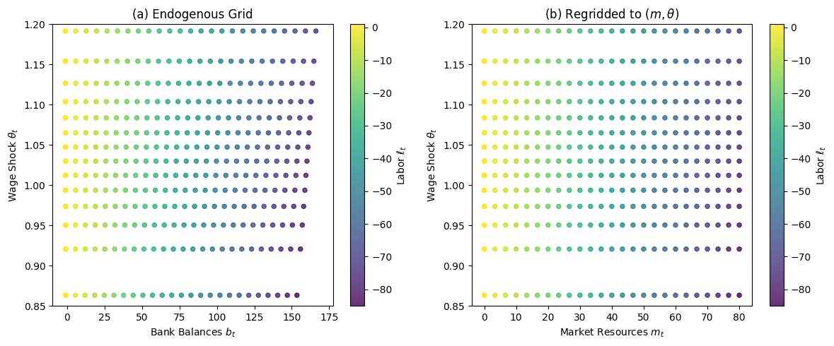

3Policy Functions¶

Let’s examine the consumption policy from the labor-leisure stage:

# Plot consumption function cross-sections for different wage shocks
plot_funcs(agent.solution_terminal.labor_leisure.c_func.xInterpolators, 0, 5)
plt.xlabel("Bank Balances $b_t$")
plt.ylabel("Consumption $c_t$")
plt.title("Consumption Policy (Terminal Period)")
plt.show()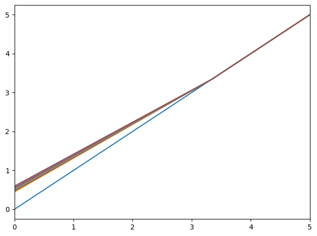

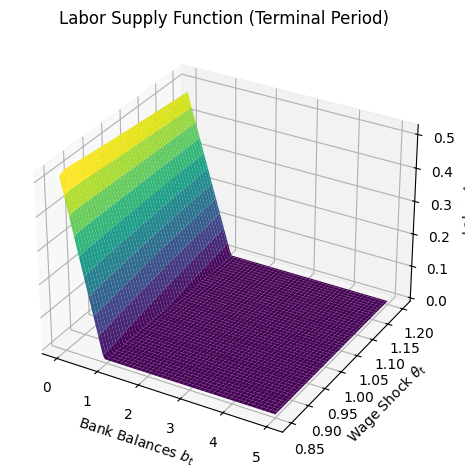
3D Policy Surfaces¶

The labor supply function depends on both bank balances and the wage shock:

plot_3d_func(
    agent.solution_terminal.labor_leisure.labor_func,
    [0, 5],
    [0.85, 1.2],
    meta={
        "title": "Labor Supply Function (Terminal Period)",
        "xlabel": "Bank Balances $b_t$",
        "ylabel": "Wage Shock $\\theta_t$",
        "zlabel": "Labor $\\ell_t$",
    },
)

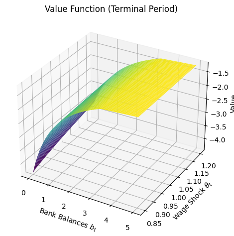
plot_3d_func(
    agent.solution_terminal.labor_leisure.v_func,
    [0, 5],
    [0.85, 1.2],
    meta={
        "title": "Value Function (Terminal Period)",
        "zlabel": "Value",
        "xlabel": "Bank Balances $b_t$",
        "ylabel": "Wage Shock $\\theta_t$",
    },
)

4Solving the Full Life-Cycle Problem¶

Now let’s solve all 10 periods via backward induction:

agent.solve()
print(f"Solved {len(agent.solution)} periods")

Solved 11 periods

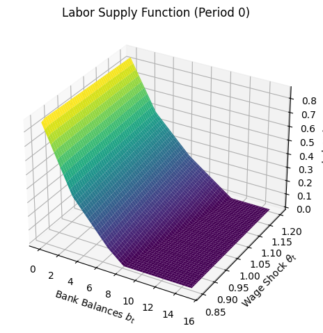
The labor function in the first period shows richer dynamics due to continuation value:

plot_3d_func(
    agent.solution[0].labor_leisure.labor_func,
    [0, 15],
    [0.85, 1.2],
    meta={
        "title": "Labor Supply Function (Period 0)",
        "xlabel": "Bank Balances $b_t$",
        "ylabel": "Wage Shock $\\theta_t$",
        "zlabel": "Labor $\\ell_t$",
    },
)

1The Model¶

2The Endogenous Grid¶

Endogenous Grid in (b,θ)(b, \theta)(b,θ) Space¶

3Policy Functions¶

3D Policy Surfaces¶

4Solving the Full Life-Cycle Problem¶

Endogenous Grid in $(b, \theta)$ Space¶