Basic Health Investment Model (HARK Baseline)
This notebook documents the BasicHealthConsumerType from HARK, a model in which agents make decisions about consumption, saving, and health investment. The model serves as the baseline against which we compare the EGM + ENGINE approach.
# Import the basic health investment consumer class, as well as some basic tools
from __future__ import annotations

from time import time

import matplotlib.pyplot as plt
import numpy as np
from HARK.ConsumptionSaving.ConsHealthModel import BasicHealthConsumerType
from HARK.utilities import plot_funcs
Background on the Model
BasicHealthConsumerType is a teaching model rather than a structural estimation tool. It demonstrates principles for solving dynamic stochastic optimization problems with multiple endogenous states and controls.
The model was originally adapted from the one in Ludwig and Schoen (Comp Econ 2018), for use by White (JEDC 2015). The version in White adds income and depreciation risk to the original Ludwig and Schoen model, and the model here very slightly adjusts how mortality works.
Ludwig & Schoen demonstrated that Delaunay triangulation can interpolate irregular endogenous gridpoints. White (2015) presented a specialized interpolation method exploiting known relationships among grid points. HARK’s default solver uses White’s method via Curvilinear2DInterp.
Model Statement
Each period , the agent experiences wage rate and health depreciation rate . The agent observes market resources and health capital , then chooses consumption and health investment . Consumption yields utility with CRRA preferences, while health investment produces additional health capital. Health is valued for two reasons: it reduces the probability of death after each period, and it increases the agent’s productivity (hence income).
The model can be expressed in Bellman form as follows:
The current solver requires (so that utility is strictly positive for all ) and , so that zero income is always possible. Combined with (so that health production is increasing and concave), these conditions guarantee that the first order conditions are necessary and sufficient for the optimal policy, and that they hold with equality.
Characterizing the Solution
As is typical in HARK, each period of this model is solved using the endogenous grid method (EGM). The end-of-period states are post-investment health capital and retained assets . Substituting the transition dynamics into the Bellman equation, the continuation value function is:
.
The Bellman form of the problem can then be expressed as:
In this representation of the model, all of the intertemporal transitions (including risk) have been wrapped up into the “gothic” value function, with only intratemporal dynamics remaining.
The first order conditions with respect to and are thus:
Rearranging terms and solving for and yields:
Inverting the intraperiod dynamics, the endogenous gridpoints associated with these optimal controls are:
To solve the model using the endogenous grid method, we must choose a grid of end-of-period states , compute end-of-period marginal value for each (with respect to both dimensions), and then apply the solution above to generate combinations of decision-time states and controls that satisfy the first order conditions. The solution to the period problem is an interpolant over those points.
The marginal value of end-of-period assets is straightforward. The marginal value of post-investment health has three terms: a marginal increase in raises survival probability (because decreases), raises income in due to higher human capital, and raises health in (with further continuation benefits). See the paper for the full derivation.
Inputs to the Solver
The solution to the terminal period is simple: the agent should consume all resources, and invest nothing in their health; the value function is simply . Each non-terminal period of the basic health investment model is solved using the function solve_one_period_ConsBasicHealth. The following objects are passed to the solver for each non-terminal period (in addition to a representation of the successor period’s solution); default values are provided:
| Param | Description | Code | Value | Constructed |
|---|---|---|---|---|
| Intertemporal discount factor | 0.95 | |||
| Coefficient of relative risk aversion | 0.5 | |||
| Risk free interest factor | 1.03 | |||
| Exponent on health production function | 0.35 | |||
| Factor on health production function | 1.0 | |||
| Maximum death probability (if ) | 0.5 | |||
| Joint dstn of wage and depreciation rates | * | |||
| Grid of end-of-period assets | * | |||
| Grid of post-investment health | * |
Objects listed as “constructed” are not specified as raw parameters, but instead built by a constructor function.
By default, the distribution of wage rate is lognormal with a point mass for unemployment, specified with parameters WageRteMean, WageRteStd, WageRteCount, UnempPrb, and IncUnemp. The distribution of depreciation rate is uniform by default, specified with parameters DeprRteMean, DeprRteSpread, and DeprRteCount. The joint distribution of shocks is assumed to be independent.
The grid of end-of-period assets has a default specification using the same constructor function as other HARK models, with the same inputs as usualt (aXtraMin, etc). The grid of post-investment health has a default specification of being uniformly distributed between hLvlMin and hLvlMax with hLvlCount nodes. Note the (lack of) capitalization, which is intentional.
Maximum death probability could be manually set as an age-varying parameter, but by default it is constructed using “logistic polynomial” coefficients. The parameter DieProbMaxCoeffs is a list representing polynomial coefficients , and the maximum death probability at each model age is constructed as:
.
This form ensures that DieProbMax is strictly between 0 and 1 for all , and that an increase in also increases . By default, DieProbMaxCoeffs = [0.0], corresponding to , as in the referenced papers.
1Example Model Solution
Let’s solve one non-terminal period of the model and then plot the resulting set of interpolating nodes.
# Make and solve an example agent type with one non-terminal period
OnePeriodExample = BasicHealthConsumerType(cycles=1)
OnePeriodExample.solve()

# Plot the interpolation nodes of its solution
X = OnePeriodExample.solution[0].x_values
Y = OnePeriodExample.solution[0].y_values
plt.plot(X.flatten(), Y.flatten(), ".k", ms=2)
plt.xlim(0.0, 100.0)
plt.ylim(0.0, 50.0)
plt.xlabel(r"Market resources $m_t$")
plt.ylabel(r"Health capital $h_t$")
plt.title(r"Endogenous gridpoints in period $T-1$")
plt.show()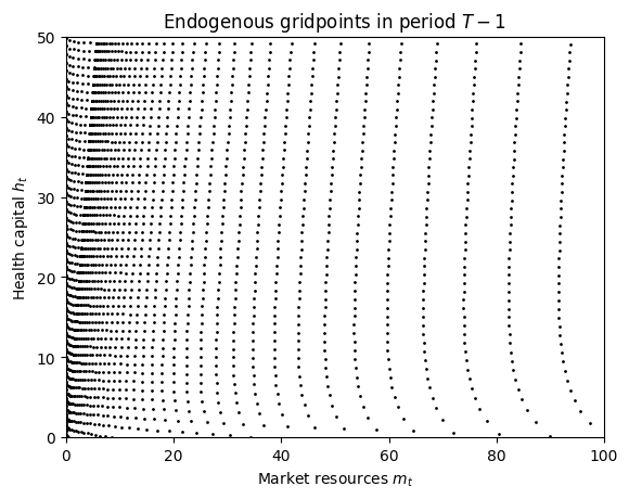
The solver represents the solution as a single interpolant with three function outputs. The endogenous gridpoints are stored in the x_values and y_values attributes.
To match what’s done in the referenced papers, let’s solve a total of 100 periods (99 non-terminal periods) and plot the gridpoints.
# Make an agent that lives for 100 periods and solve their problem; this will take a moment
BasicHealthExample = BasicHealthConsumerType(cycles=99)
t0 = time()
BasicHealthExample.solve()
t1 = time()
# Plot the interpolation nodes of its solution at t=0
X = BasicHealthExample.solution[0].x_values
Y = BasicHealthExample.solution[0].y_values
plt.plot(X.flatten(), Y.flatten(), ".k", ms=2)
plt.xlim(0.0, 100.0)
plt.ylim(0.0, 50.0)
plt.xlabel(r"Market resources $m_t$")
plt.ylabel(r"Health capital $h_t$")
plt.title(r"Endogenous gridpoints in period $t=0$")
plt.show()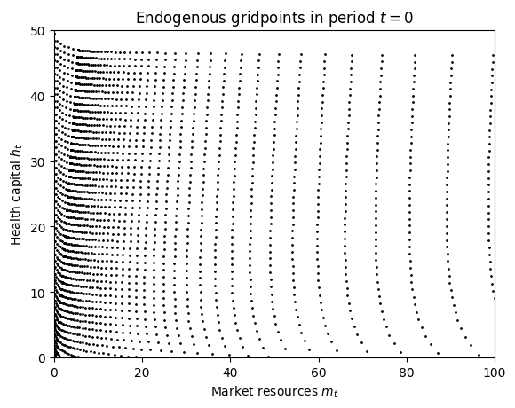
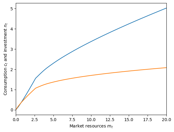
Now let’s plot some cross sections of its policy functions. In the cell below, the function output indexed by [1] is consumption and the output indexed by [2] is health investment.
# Define cross sections of the consumption and health investment functions
t = 0
hLvl = 20.0


def C(mLvl):
    return BasicHealthExample.solution[t](mLvl, hLvl * np.ones_like(mLvl))[1]


def N(mLvl):
    return BasicHealthExample.solution[t](mLvl, hLvl * np.ones_like(mLvl))[2]


# Now plot them in a simple figure
plt.xlabel(r"Market resources $m_t$")
plt.ylabel(r"Consumption $c_t$ and investment $n_t$")
plot_funcs([C, N], 0.0, 20.0)