Part A specifies the health-investment interpolation testbed and its warp sweep; Part B reports the full-solve interpolation diagnostic’s protocol and readings. Section references point to the main paper.
The Health Investment Model as an Interpolation Testbed
The two-asset household block of Section 3 is the paper’s primary multidimensional application. For two reasons, this appendix retains a second two-dimensional model, the consumption-saving problem with health investment of Ludwig & Schön (2018) extended with the wage and depreciation risk of White (2015). First, the model is home ground for both alternatives: Ludwig & Schön (2018) introduced Delaunay interpolation on the version whose only risk is survival, and White (2015) introduced curvilinear interpolation on the stochastic version adapted here. Second, the health-investment stage is a concrete instance of the invertible-transition-marginal form of the paper’s Section 5.
A Health Investment Model
Each period , the household observes market resources and health capital and chooses consumption and health investment . Consumption yields CRRA utility; health investment produces health capital through a concave production function; and health capital both reduces mortality risk and raises labor income.
The recursive problem is
where the utility function and health production function are
Here is post-investment health capital, end-of-period assets, the survival probability (the maximum death probability applies at ), the stochastic health depreciation rate, the stochastic wage rate, and labor income. Ludwig & Schön (2018) take this survival function from Hall & Jones (2007). With scale and elasticity , health investment has diminishing returns. The terminal condition makes the final-period household consume all remaining resources. Higher health investment raises and thereby the weight on future value.
This model requires , so utility is non-negative for all . With a positive probability of zero wage, ending a nonterminal period with no liquid assets would risk zero consumption, so the liquidity constraint never binds before the terminal period. Strict concavity then makes the first-order conditions necessary and sufficient at interior solutions. The implementation also handles positive wage floors, like the benchmark calibration’s unemployment-income floor, through an explicit liquidity-constrained segment at . As , approaches a constant, the marginal inversion becomes ill-conditioned, and at the linear limit the first-order condition no longer identifies health investment. This boundary case therefore falls outside the invertible-transition-marginal class.[1]
Sequential EGM Solution
The problem splits into three stages: health investment, consumption, and a post-decision stage that handles expectations. I retain the stage superscripts of Section 2, so is the first decision stage, and write in place of for the post-decision value, following Powell (2011). Because value functions have multiple arguments, partials appear as superscripts ().
The post-decision stage values the end-of-period states before next period’s shocks are realized:
Building once lets the earlier stages reuse it without repeated expectation calculations.[2]
After the health investment decision, the household has liquid wealth and post-investment health . The consumption problem is
Post-investment health passes through this stage because it enters the continuation value and the consumption decision leaves it unchanged. For each fixed , this is a standard one-dimensional consumption-saving problem that EGM solves.[3] On an exogenous grid of post-decision states, the first-order condition inverts to , which defines the endogenous liquid-wealth grid . On that grid the envelope conditions give the investment stage the marginal values and .
At the beginning of the period, the household has market resources and health capital . The health investment problem is
With no direct utility payoff at this stage, investment moves liquid wealth through the budget and post-investment health through the production function. Because has an explicit inverse, the EGM step can run before the transition equations recover the incoming states. The Inada condition handles the constraint , keeping solutions interior whenever the marginal value of health is positive and resources permit.
The first-order condition of the health investment problem rearranges to
Since is strictly decreasing for , optimal health investment on an exogenous grid of liquid wealth and post-investment health follows:
From the transition equations, the endogenous pre-decision states then follow:
By the envelope theorem, the beginning-of-period marginal values are
Starting from a regular rectilinear grid of , the two EGM steps together produce the curvilinear endogenous grid of shown in Figure 1.[4]
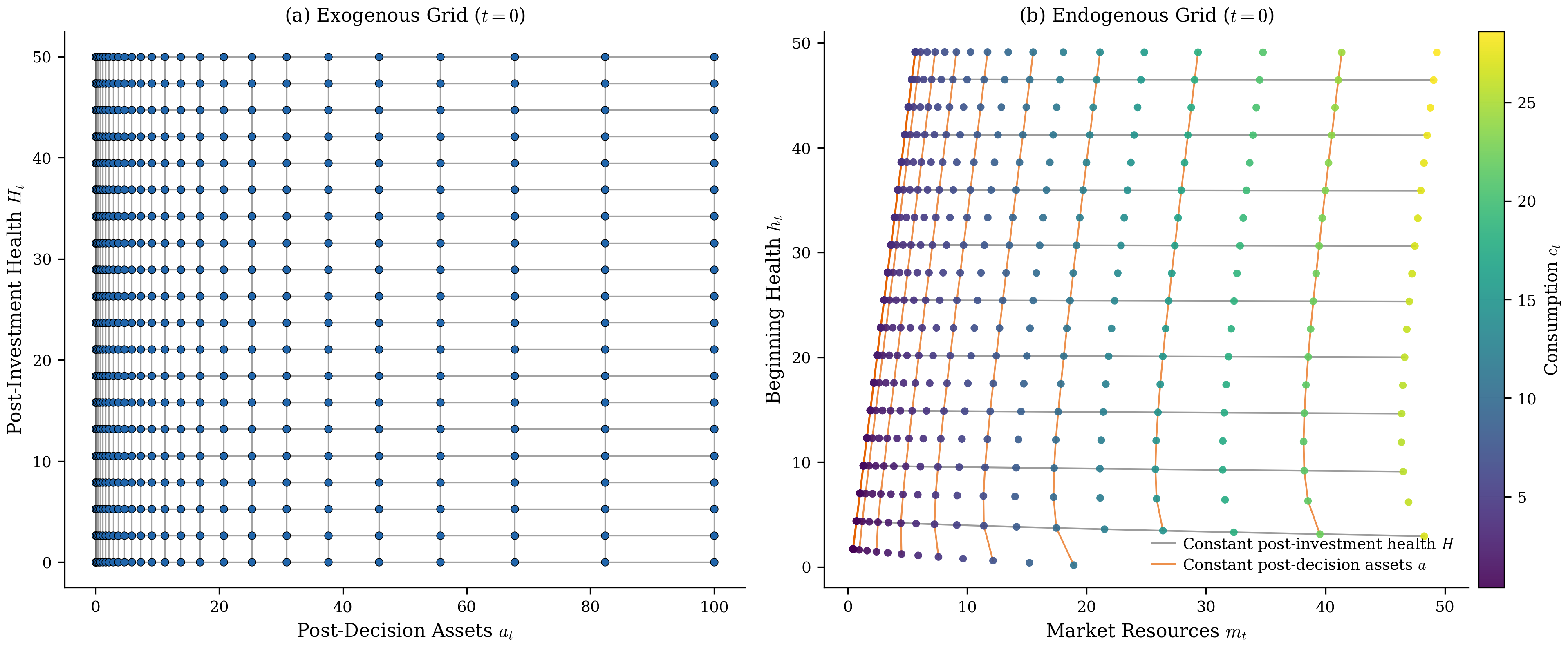
Figure 1:EGM grid transformation for the health investment model at (the first period of economic life). Panel (a) shows the regular exogenous grid of post-decision assets and post-investment health . Panel (b) shows the curvilinear endogenous grid of market resources and beginning-of-period health , with points colored by optimal consumption and the plot windowed to for legibility. The endogenous grid preserves the index ordering of the exogenous grid despite substantial warping near the constraint boundary.
Index preservation across warping enables the interpolation strategy of Section 4. The mapping above is the recovery map whose sampled meshes the warp sweep below measures.
Interpolation Comparison
This appendix adds Delaunay triangulation to the comparison of Section 4, on a model where all three methods complete. Figure 2 times the two structured methods across both time horizon (backward-induction cycles) and grid resolution.[5] Apart from one small grid, the grid sweep holds fifty health nodes and scales the asset axis from 44 to 176 points; the cycle sweep stops at fifteen cycles. Denser health grids or twenty cycles make the endogenous health coordinate non-monotone between the two lowest health nodes, which violates IPM, a condition ENGINE requires. On this model the comparison isolates the interpolation method cleanly, because the sequential and simultaneous solvers produce numerically identical policies (the maximum absolute difference in consumption is ). EGM with ENGINE solves 2.8 to 4.7 times faster than the simultaneous solver with the curvilinear method across both sweeps. A third configuration that swaps only the interpolant on the simultaneous solver reproduces most of that gap, so the interpolation method, not the decomposition, accounts for the bulk of the speedup.
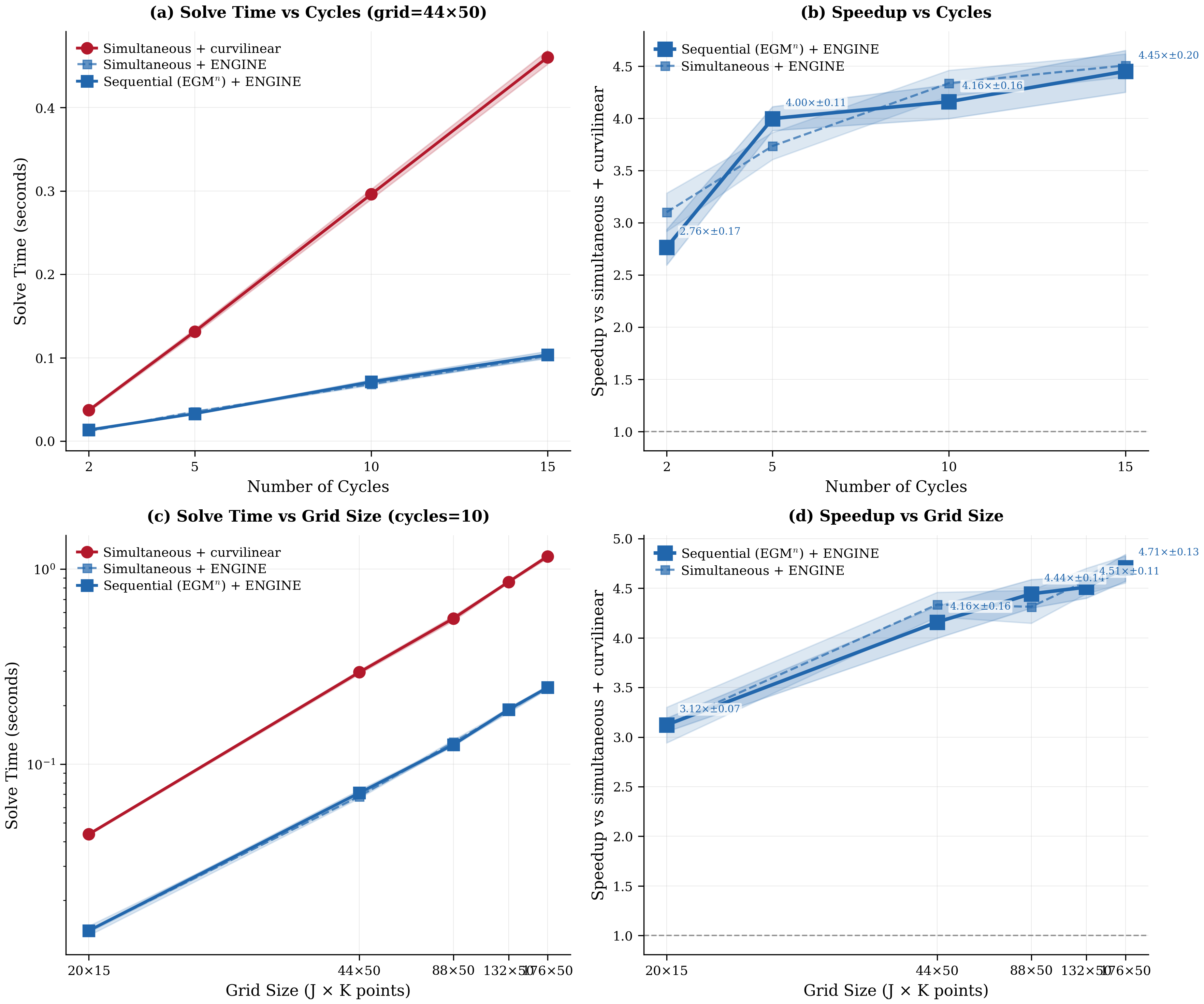
Figure 2:Solve time and speedup on the health investment model, by backward-induction cycles at a grid (a, b) and by grid size at ten cycles (c, d). Annotations give the speedup of EGM with ENGINE over the simultaneous solver with the curvilinear method of White (2015). Bands are 95 percent confidence intervals of the mean over ten timed runs.
The converged policies separate the structured methods from the triangulation just as the timings do. Each interpolation method runs inside its own backward solve (holding the simultaneous solver fixed), and interpolation differences propagate through the solution. On a uniform grid of off-mesh query points spanning , with the curvilinear solution as the reference, ENGINE differs by a mean of in consumption (maximum ) and in health investment (maximum ); Delaunay triangulation differs by means of and (maxima and ).
Figure 3 maps the consumption disagreement over the state space. ENGINE’s differences from the curvilinear solution are small and nearly uniform, between 10-8 and 10-4 over most of the domain. However, the worst case, , occurs in the few visible spots at the lowest market resources where the mesh cells are most warped, with fainter disagreement at the lowest health capital. The triangulation’s differences are larger and spatially diffuse, following its simplex boundaries.
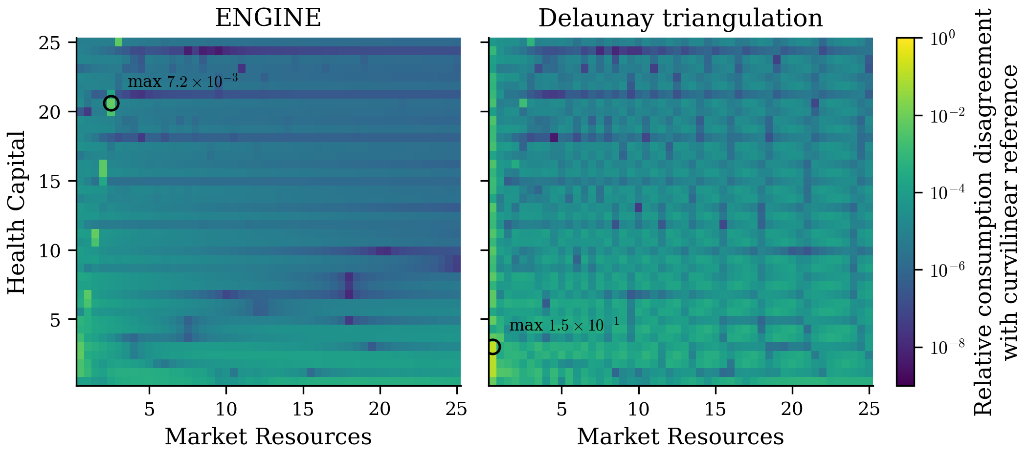
Figure 3:Consumption disagreement with the curvilinear reference over the query plane, on a shared logarithmic color scale. (Left) ENGINE. (Right) Delaunay triangulation. Circles mark each panel’s maximum.
Accuracy against Measured Warp
The comparison above fixes the calibration and varies the query point. How do the methods behave as the mesh itself becomes more warped? I vary the two model parameters that bend the endogenous mesh hardest. Across the sweep, the health production elasticity takes values in , controlling the curvature of the investment inversion, and the maximum death probability , held constant across ages in every sweep calibration, takes values in , scaling the survival term in . I solve each of the nine calibrations for five periods on a smaller grid under the protocol above (each interpolant inside its own backward solve, with the simultaneous solver held fixed). After every solve I test IPM slice by slice and measure the warp by the empirical constant of Section 4, the maximum bracket displacement between adjacent health slices.
Accuracy is scored against the model’s own optimality conditions rather than against any reference solution. At three thousand off-mesh query points I rebuild the post-decision marginals and by quadrature through the true continuation solution and evaluate both first-order conditions. The consumption Euler residual uses implied consumption capped at the budget bound, so constrained queries are scored rather than discarded. The investment margin holds at interior investment whether or not the liquidity constraint binds, since the Inada condition on keeps investment interior. Queries where an interpolated policy violates feasibility, whether through the budget or through a negative control, are repaired minimally for the quadrature and counted, none of them dropped.
Every warp-sweep mesh the two structured methods produce satisfies IPM. Yet across those meshes ranges from 10 to 16, five to eight times ENGINE’s default search margin of two. A mismatch in grid spacing produces these values: twenty health nodes span whereas the asset axis is finely log-spaced, so a query’s bracket can cross many asset cells between adjacent health slices. Without the containment fallback of Section 4, the default-margin search misses brackets on this sweep without raising an error, producing budget-infeasible interpolated policies and inflated extreme residuals. Setting the margin to the measured constant removes every violation on the sweep’s declared finite query set at no measurable time cost. All sweep solves use that matched margin. The archived implementation also carries the fallback, which runs a full row search when a windowed bracket misses the query.
Every fold on the structured meshes is a sliver cell at the lowest post-decision health node. I start the health grid at . The HARK implementation of this model starts it at zero, where the investment inversion at zero assets divides one infinite marginal value by another. At , however, the investment the inversion assigns, even at zero assets, produces more health than the node holds, so every inverted state on that row has negative health and lies outside the state space. Whether a cell on that row folds depends on the calibration, so I count the folds directly. The final period, inverted on the analytic terminal solution with no interpolation, produces the same slivers. Evaluation points reach the cells only at and . There, up to 0.45 percent of continuation points fall in folded cells, and at so do 0.37 percent of final queries for the curvilinear method and 0.40 percent for ENGINE. Although ENGINE’s fold-free requirement fails in those cells, the reported residuals include every query inside one.
The triangulation’s own meshes violate IPM at five of the nine calibrations, the three with the lowest production elasticity (0.20) and the other two with the highest mortality (0.82). At the remaining four the triangulation’s is 12 or 13, against 10 to 12 for the structured meshes. In each of the five, between 82 and 120 of the mesh’s 820 nodes are undefined. The continuation queries of the highest health node fall above the convex hull of the next period’s mesh, where the boundary triangles stretch to outlying mesh nodes, and linear extrapolation from those triangles returns values outside the admissible range, such as negative consumption. The first-order conditions are then undefined for that health column, whose nodes drop out of the next triangulation. As the hull shrinks, the undefined nodes spread one period back at a time. By contrast, the two structured methods extrapolate along the mesh’s own index lines; every node of their meshes is defined at all nine calibrations.
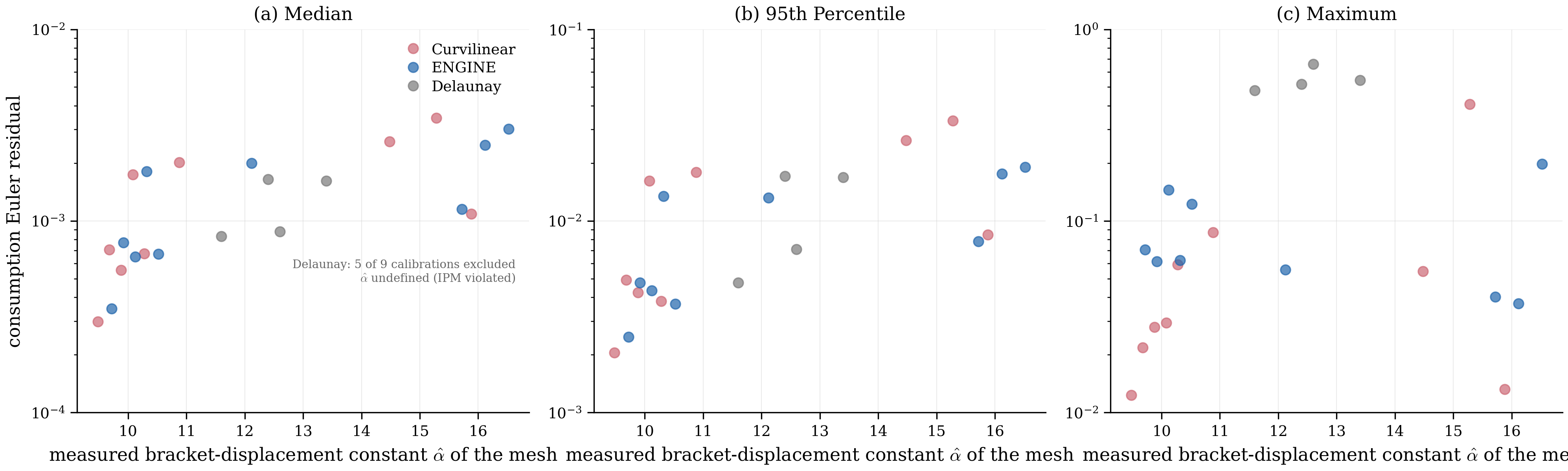
Figure 4:Consumption Euler residuals at off-mesh queries (median, 95th percentile, and maximum) against the measured bracket-displacement constant of each solve’s own endogenous mesh, across nine calibrations varying the production elasticity and the maximum death probability. Markers are horizontally jittered for legibility, and the three panels use different vertical scales; the triangulation’s five IPM-violating meshes have no defined and are absent from the panels.
Figure 4 reports the consumption residuals against this measured warp. Median accuracy, between and across the sweep, moves by an order of magnitude with the calibration but by less than a factor of two across methods at any single calibration. The interpolant therefore matters far less for the median than the calibration’s warp does at this grid resolution.
The triangulation’s maximum residual sits between 0.25 and 0.66 at every calibration, including the five IPM-violating meshes the figure cannot place, repeating the simplex-boundary artifacts in Figure 3. ENGINE has both a smaller 95th-percentile and a smaller maximum consumption residual than the curvilinear method in exactly three calibrations: . At the last of these, its two consumption statistics, 0.019 and 0.20, are below the curvilinear method’s 0.033 and 0.41, and its maximum investment residual falls from 0.60 to 0.15. The constant alone does not rank the tails: among the three calibrations where ENGINE’s mesh has , ENGINE’s maximum consumption residual is higher at , lower at , and roughly half as large only at . Across the full sweep, ENGINE’s 95th percentile is smaller at seven of nine calibrations.
Every solve in the sweep completes. I compare timings only on the larger grids of Figure 2.
The Full-Solve Interpolation Diagnostic
This appendix records the protocol behind Section 4’s full-solve-time comparison of ENGINE with the sector-walking curvilinear method of White (2015). Online Appendix A adds the Delaunay triangulation of Ludwig & Schön (2018).
I solve the Section 3 household block with each interpolator as the Stage-0 realign step, holding every other component fixed. Productivity follows the same three-state Rouwenhorst chain in every solve, with persistence 0.966 and unconditional standard deviation 0.92 for log productivity. Each iteration starts from the same marginal-value initialization and stops when the larger normalized sup-norm change in the beginning-of-period marginal values and (the arrays Va and Vb of the replication code) falls below 10-9, subject to a cap of backward steps; the normalization for either marginal is one plus the sup norm of its previous iterate. At coarse (), medium (), and fine () grids, both methods use linear interpolation and sixteen Numba threads. Solve time is the best of three repetitions after a separate warm-up, so compilation is excluded. The residual compares consumption with the minimum of the Euler-implied and binding-constraint levels at off-grid queries, so no constraint-bound query is excluded. The queries are the axis midpoints below 85 percent of each grid maximum, crossed over both states and every income state.
Both solves use the same regular-grid Euler inversion. On the endogenous mesh, Stage 1 selects , inverts to , and obtains . On the regular pre-decision grid the solver again inverts the Euler equation on the interpolated continuation marginal, rather than interpolating the kinked consumption policy. With fixed, the Stage 1 policy supplies the evaluation point. One application of the inversion matches NEGM and the curvilinear interpolant off-grid, whereas a second, diagnostic application lowers on-grid Euler residuals to 10-6 to 10-7 without changing off-grid accuracy.
The grid axes are the model’s own log-spaced asset grids, which concentrate points near the borrowing constraints. The diagnostic therefore exercises the mesh conditions on strongly non-uniform spacing by construction rather than on uniform grids, which are probably the most favorable to them. Each method runs with its native boundary behavior, so neither receives an out-of-hull correction. To measure how often that behavior is used, I classify every regular Stage-0 target at the converged fixed point as inside or outside the polygon bounded by the verified fold-free bilinear mesh. Table 1 reports the pooled count over all three income states at each grid. The replication CSV also reports each income state separately. Boundary points count as interpolation, so the reported outside share measures boundary-slope extrapolation rather than contact with the mesh boundary.
Table 1:Stage-0 extrapolation frequency at the converged fixed point: regular targets outside the endogenous mesh, pooled over income states. Boundary points count as interpolation.
| Grid | Outside / total | Outside (percent) |
| 1 / 1440 | 0.069 | |
| 1 / 5760 | 0.017 | |
| 1 / 23040 | 0.004 |
Only one target lies outside the mesh at every resolution. Because the number of targets grows with the grid, the outside share falls from 0.069 to 0.004 percent. This is a fixed-point result only; the iteration path was not recorded.
ENGINE’s median robust Euler error falls from -1.79 to -2.47 to -3.14, about fivefold per grid doubling. The 95th percentile remains four to six times the median, and the fine-grid worst-query error is below 1 percent. Both structured interpolants reach these levels on this metric, so linear interpolation at these grid densities probably sets them on this model, in which each of the two stacked first-order conditions uses marginal values interpolated at off-grid midpoints. Inside the 85-percent interior query set, both passes bracket rather than extrapolate. In the complementary high-wealth band, the worst residual improves monotonically from -1.08 to -1.69 to -2.32 in units. The band median, however, is not monotone, moving from -2.24 to -1.74 before falling to -2.75. At every resolution the band maximum is no larger than the interior maximum to within a fraction of a percent, with the two methods within one percent of each other.
With a solution as the benchmark, median consumption-policy error falls from 9.3 to 3.7 to 0.9 percent and the worst query from 18 to 3.3 percent. The median robust Euler residual is about six to twelve times smaller than the median policy error because the policy is locally optimal given its grid’s continuation value. Extending both state-grid maxima by half barely moves the typical medium-grid policy (a median of 0.05 percent), but the 4.3 percent maximum rules out treating grid placement as irrelevant at every query. Table 2 reports both checks.
Table 2:Consumption-policy refinement and upper-bound sensitivity, as relative differences in percent over a common set of coarse-grid interior midpoints and all income states. Refinement rows compare each grid with the benchmark; the bounds row compares the medium grid with both state-grid maxima scaled by 1.5.
| Exercise | Grid | Median | p95 | Maximum |
| Refinement | 9.25 | 17.84 | 18.47 | |
| Refinement | 3.69 | 8.35 | 8.75 | |
| Refinement | 0.89 | 2.77 | 3.31 | |
| Bounds | 0.05 | 0.39 | 4.27 |
Section 4’s pass-order reversal comparison uses this same protocol, with each pass order solved to convergence; the replication archive records its results at every grid.
The component table (Table 3) assigns about one percent of serial time to expectations, a little over one third to the two stage inversions, five percent to ENGINE, and the remainder to the regular-grid Euler inversion and envelope updates. Components are timed on one thread at the Section 3 grids with the full-solve diagnostic’s code, whose ENGINE configuration reproduces the paper’s EGM solver exactly. Summed, they track Section 3’s timings within two percent at every grid.
Table 3:Runtime in seconds by component of the EGM backward solve, summed over a converged one-thread solve (shares in parentheses). Stage inversions are Stage 1’s consumption EGM and the Stage 0 inversion; mesh-to-grid interpolation is the ENGINE regrid; regular-grid inversion is corner selection, Euler inversion, and envelope updates.
| Grid | Expectation | Stage inversions | Mesh-to-grid | Regular-grid inversion |
| 0.01 (1%) | 0.28 (36%) | 0.04 (5%) | 0.45 (58%) | |
| 0.03 (1%) | 1.15 (35%) | 0.15 (5%) | 1.92 (59%) | |
| 0.10 (1%) | 4.67 (35%) | 0.63 (5%) | 8.09 (60%) |
The Auclert et al. (2021) block also has a native hybrid NEGM/G2EGM solver, at the version pinned in the replication archive. At matched grids and tolerance (Table 4), EGM uses fewer iterations (395 to 424 versus 464 to 478) and has off-grid robust Euler medians within fifty percent of the native solver’s, smaller at the smallest grid and larger at the two finer grids. The native solver’s distributed array code runs 3.0 to 4.6 times faster than one-thread EGM, while sixteen-thread EGM is about five percent faster on the coarse grid and faster by factors of 1.4 and 1.7 on the two finer grids. Its EGM times, from a separate run of the configuration in Table 1, lie within three percent of that table’s. The native benchmark does not isolate the method. For that comparison, Section 3 uses NEGM with matched threading and shared components.
Table 4:Time in seconds and converged-policy accuracy: the two-asset block’s native solver versus EGM, at matched grids, tolerance, and linear interpolation. The native solver is serial; parentheses give its time over EGM’s at sixteen threads. Iterations are backward steps to the shared tolerance; accuracy is the off-grid robust Euler median (), EGM first.
| Grid | Native, serial | EGM | Iterations | Accuracy | |
| 1 thread | 16 threads | EGM/native | EGM/native | ||
| 0.25 | 0.76 | 0.24 (1.1x) | 395/478 | -2.86/-2.78 | |
| 0.78 | 3.22 | 0.55 (1.4x) | 410/467 | -3.44/-3.58 | |
| 2.94 | 13.41 | 1.74 (1.7x) | 424/464 | -4.21/-4.36 | |
With , utility is negative and the product would reward mortality. The restriction mirrors the calibrations of Ludwig & Schön (2018) and White (2015) and is specific to this health formulation, not to EGM generally. Models with mortality risk and can use a bequest motive or utility differences (see De Nardi (2004)).
The marginal value functions and are computed once on an exogenous grid and interpolated as needed by earlier stages. The health marginal includes both the survival-probability benefit of health (through ) and the continuation-value benefit through next period’s health.
Strict concavity of and ensures joint strict concavity of , so the recovered optimum is unique. Grid validity is separate: concavity alone does not deliver fold-freeness or index monotonicity, so the warp sweep below tests both directly on every solved mesh.
The figure uses , , , health production exponent , health depreciation rate , wage rate with mean 0.1 and standard deviation 0.1, and a two-period model (, so the household lives periods ).
The two codebases are compiled alike (Section 4’s implementation footnote) and run on the same hardware and software as Section 3’s benchmarks, both recorded in the replication archive’s README.
- Ludwig, A., & Schön, M. (2018). Endogenous Grids in Higher Dimensions: Delaunay Interpolation and Hybrid Methods. Computational Economics, 51(3), 463–492. 10.1007/s10614-016-9611-2
- White, M. N. (2015). The method of endogenous gridpoints in theory and practice. Journal of Economic Dynamics and Control, 60, 26–41. 10.1016/j.jedc.2015.08.001
- Hall, R. E., & Jones, C. I. (2007). The Value of Life and the Rise in Health Spending. The Quarterly Journal of Economics, 122(1), 39–72. 10.1162/qjec.122.1.39
- Powell, W. B. (2011). Approximate Dynamic Programming: Solving the Curses of Dimensionality (2nd ed.). Wiley. 10.1002/9781118029176
- Auclert, A., Bardóczy, B., Rognlie, M., & Straub, L. (2021). Using the Sequence-Space Jacobian to Solve and Estimate Heterogeneous-Agent Models. Econometrica, 89(5), 2375–2408. 10.3982/ECTA17434
- De Nardi, M. (2004). Wealth Inequality and Intergenerational Links. The Review of Economic Studies, 71(3), 743–768. 10.1111/j.1467-937X.2004.00302.x