Consumption-Labor Choice with Sequential EGM

This notebook solves the consumption-labor model of Section 2, the paper’s smallest example of chaining two EGM inversions in one period, and then extends it with a risky portfolio share. The extension adds a stage that has no closed-form inversion. Its solution uses the numerical fallback of Section 5, while the labor and consumption stages run exactly as they do in the two-stage model.

import sys

sys.path.append("../")
sys.path.append("../figures")

import matplotlib.pyplot as plt
import numpy as np
from cli import format_table
from figure_styles import apply_engine_style
from generate_consumption_labor_figure import (
    mpc_csv_rows,
    plot_consumption_by_age_panel,
    plot_endogenous_grid_panel,
    plot_leisure_by_wage_panel,
)
from HARKmodels.ConsLaborPortfolioModel import (
    LaborPortfolioConsumerType,
    LaborPortfolioSolver,
    portfolio_residuals,
)
from HARKmodels.ConsLaborSeparableModel import (
    LaborSeparableConsumerType,
    LaborSeparableSolver,
    consumption_euler_residual,
    labor_utility_funcs,
    make_labor_separable_solution_terminal,
)
from repo_paths import FIG_DIR, read_rows

apply_engine_style()

1The Household Problem¶

A household enters period $t$ with liquid assets $a_{t}$ and draws a transitory wage $θ_{t}$ . It chooses leisure $z_{t} \in [0, 1]$ , so that it works $n_{t} = 1 - z_{t}$ , and then consumption $c_{t}$ , with

m_{t} = 𝖱 a_{t} + θ_{t} n_{t}, a_{t + 1} = m_{t} - c_{t},

(1)

and period utility $u (c) + h (z) = c^{1 - ρ} / (1 - ρ) + ν z^{1 - ζ} / (1 - ζ)$ . Section 2 orders the period in three stages, each with its own value function:

\begin{matrix} v_{t}^{0} (a_{t}, θ_{t}) & = \max_{z_{t} \in [0,1]} h (z_{t}) + v_{t}^{1} (m_{t}), \\ v_{t}^{1} (m_{t}) & = \max_{c_{t} \in [0, m_{t}]} u (c_{t}) + v_{t}^{2} (a_{t + 1}), \\ v_{t}^{2} (a_{t + 1}) & = β 𝔼_{t} [v_{t + 1}^{0} (a_{t + 1}, θ_{t + 1})] . \end{matrix}

(2)

Placing the labor stage first resolves the wage before the consumption stage, which then keeps a single state. In the code, the labor stage takes as its state the bank balance $b_{t} = 𝖱 a_{t}$ , the incoming assets with their return. Market resources are $m_{t} = b_{t} + w θ_{t} n_{t}$ with the wage rate $w = 1$ . HARK also multiplies $β$ by a survival probability. The calibration below is that of the paper’s figure.

agent = LaborSeparableConsumerType(cycles=30)
nu = agent.LeisureFactor ** (1 - agent.CRRA)  # h(z) = nu z^(1 - zeta) / (1 - zeta)
print(
    format_table(
        ["Parameter", "Value"],
        [
            ["Relative risk aversion (rho)", agent.CRRA],
            ["Discount factor (beta)", agent.DiscFac],
            ["Survival probability", agent.LivPrb[0]],
            ["Risk-free return (R)", agent.Rfree[0]],
            ["Leisure curvature (zeta)", agent.LeisureCRRA],
            ["Leisure weight (nu)", nu],
            ["Wage shock dispersion", agent.TranShkStd[0]],
            ["Zero-wage probability", agent.UnempPrb],
            ["Wage rate (w)", agent.WageRte[0]],
            ["Decision periods", agent.cycles],
        ],
    )
)

Parameter                     Value
----------------------------  -----
Relative risk aversion (rho)  5.0
Discount factor (beta)        0.9
Survival probability          0.98
Risk-free return (R)          1.03
Leisure curvature (zeta)      2.0
Leisure weight (nu)           16.0
Wage shock dispersion         0.1
Zero-wage probability         0.05
Wage rate (w)                 1.0
Decision periods              30

2Two Inversions¶

The consumption stage is the standard EGM of Carroll (2006). On an exogenous grid of end-of-period assets, inverting the Euler equation $u^{'} (c_{t}) = {(v_{t}^{2})}^{'} (a_{t + 1})$ gives consumption, and the budget gives the endogenous market resources $m_{t} = c_{t} + a_{t + 1}$ . The labor stage applies the same idea to leisure. Its first-order condition $h^{'} (z_{t}) = {(v_{t}^{1})}^{'} (m_{t}) θ_{t}$ inverts in closed form,

z_{t} = (h^{'})^{- 1} ((v_{t}^{1})^{'} (m_{t}) θ_{t}) = {(\frac{(v_{t}^{1})^{'} (m_{t}) θ_{t}}{ν})}^{- 1 / ζ},

(3)

on an exogenous grid of $(m_{t}, θ_{t})$ , after which the budget returns the endogenous bank balance $b_{t} = m_{t} - θ_{t} n_{t}$ . Where the inverted leisure exceeds the time endowment, the solver projects it onto $z_{t} = 1$ .

After the solve, one node of the first-period labor stage shows the inversion at work. At that node the leisure the solver stored matches the closed form above and satisfies the first-order condition, while the stored bank balance is the budget identity.

agent.solve()
sol = agent.solution[0]
u_func, h_func = labor_utility_funcs(
    agent.CRRA,
    agent.Disutility,
    agent.LaborCRRA,
    agent.LaborFactor,
    agent.LeisureCRRA,
    agent.LeisureFactor,
)
grids = sol.labor_leisure.grids
i, j = np.searchsorted(grids["mNrm"][:, 0], 2.0), grids["tShk"].shape[1] // 2
m_node, theta_node = grids["mNrm"][i, j], grids["tShk"][i, j]
target = sol.consumption_saving.vp_func(m_node) * agent.WageRte[0] * theta_node
z_closed = (target / nu) ** (-1 / agent.LeisureCRRA)
print(f"node: m = {m_node:.4f}, theta = {theta_node:.4f}")
print(f"stored leisure      z = {grids['leisure'][i, j]:.15f}")
print(f"closed form         z = {z_closed:.15f}")
print(f"h'(z)                 = {h_func.der(grids['leisure'][i, j]):.15f}")
print(f"v1'(m) theta          = {target:.15f}")
print(f"stored bank balance b = {grids['bNrm'][i, j]:.15f}")
print(f"m - theta n           = {m_node - theta_node * grids['labor'][i, j]:.15f}")

node: m = 2.0196, theta = 1.0474
stored leisure      z = 0.751797789658500
closed form         z = 0.751797789658500
h'(z)                 = 28.308567520812279
v1'(m) theta          = 28.308567520812275
stored bank balance b = 1.759620466390091
m - theta n           = 1.759620466390091

3Solving the Model¶

agent.solve() above ran the backward recursion over all 30 periods. A direct check of the result is the consumption Euler equation, with next period’s consumption composed through both stages, first the labor policy at $b_{t + 1} = 𝖱 a_{t + 1}$ and then the consumption policy at the market resources that labor choice produces. consumption_euler_residual returns the relative consumption error $\hat{c} / c - 1$ , where $\hat{c}$ inverts the right-hand side of the Euler equation.

m_check = np.linspace(0.3, 10.0, 200)
residual = consumption_euler_residual(agent, m_check)
print(f"largest |c_Euler / c - 1| on m in [0.3, 10]: {np.abs(residual).max():.1e}")

largest |c_Euler / c - 1| on m in [0.3, 10]: 1.5e-04

Between nodes, the composition evaluates two piecewise linear policies. If interpolation accounts for the residual, it should shrink as the asset grid is refined. Solving again on 48, 96 and 192 asset-grid points shows that it does:

refine_rows = []
for n_a in (48, 96, 192):
    coarse = LaborSeparableConsumerType(cycles=30, aXtraCount=n_a)
    coarse.solve()
    refine_rows.append([n_a, f"{np.abs(consumption_euler_residual(coarse, m_check)).max():.1e}"])
print(format_table(["Asset-grid points", "Largest |c_Euler / c - 1|"], refine_rows))

Asset-grid points  Largest |c_Euler / c - 1|
-----------------  -------------------------
48                 3.5e-03
96                 6.2e-04
192                1.5e-04

Each doubling of the asset grid cuts the largest residual by roughly a factor of four.

4The Endogenous Grid and the Policies¶

Below, the paper’s figure is redrawn from this solve. Panel (a) is the endogenous grid of the first-period labor stage, on which each exogenous node $(m, θ)$ lands at the bank balance its labor choice implies. Panel (b) shows consumption at every age except the last two, and panel (c) the first-period leisure policy at six wage draws.

fig = plt.figure(figsize=(16, 4.8))
ax_grid = fig.add_subplot(1, 3, 1)
plot_endogenous_grid_panel(ax_grid, sol)
ax_grid.set_xlabel(r"Bank Balance $b_t = \mathsf{R} a_t$")
plot_consumption_by_age_panel(fig.add_subplot(1, 3, 2), agent)
plot_leisure_by_wage_panel(fig.add_subplot(1, 3, 3), sol)
plt.tight_layout(pad=1.5)
plt.show()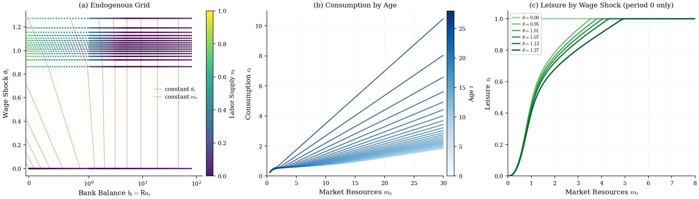

Each wage draw keeps its own row of nodes, while the warping shows in the lines of constant $m$ . Along one of them, a higher wage raises labor income $θ n$ , since panel (c) shows leisure falling as the wage rises. The same market resources then come from a smaller bank balance, which tilts the line to the left. At high market resources leisure is at its bound. Labor income is then zero, $b = m$ , and the line is vertical. The zero-wage household stays at full leisure throughout.

The text of Section 2 quotes the first-period marginal propensity to consume and the household’s expected future labor. Both come from consumption_labor_mpc.csv, which the figure script writes. This run recomputes each row with the same functions:

rows = mpc_csv_rows(agent)
published = {(r["quantity"], float(r["m"])): float(r["value"]) for r in read_rows(FIG_DIR / "consumption_labor_mpc.csv")}
print(
    format_table(
        ["Quantity", "m", "This run", "Published"],
        [[q, f"{m:.4g}", f"{v:.6g}", f"{published[q, float(f'{m:.4g}')]:.6g}"] for q, m, v in rows],
    )
)

Quantity                 m      This run   Published
-----------------------  -----  ---------  ---------
mpc_first_segment        0      0.47686    0.47686
mpc_at_m                 0.5    0.456941   0.456941
mpc_trough               4.416  0.0243734  0.0243734
mpc_plateau              22.5   0.0609332  0.0609332
future_labor             2      11.045     11.045
future_labor             7      6.77008    6.77008
future_labor             13     1.70092    1.70092
future_labor             16     0.127776   0.127776
future_labor             20     0          0
future_labor_first_zero  17.75  0          0

The propensity to consume falls from near one half at the borrowing constraint to a trough near $m = 4.4$ and then rises slowly. Expected future labor, summed over the remaining periods along the simulated savings path, declines from about 11 periods’ worth at $m = 2$ and first reaches zero near $m = 18$ (the future_labor_first_zero row, found on a grid of step 0.25).

Now give the household a risky asset with gross return ${\tilde{𝖱}}_{t + 1}$ alongside the safe one, and let it choose the risky share $ς_{t} \in [0, 1]$ of its end-of-period assets. The new choice is a stage of its own, placed after consumption, where the only state is $a_{t + 1}$ :

\begin{matrix} v_{t}^{2} (a_{t + 1}) & = \max_{ς_{t} \in [0,1]} v_{t}^{3} (a_{t + 1}, ς_{t}), \\ v_{t}^{3} (a_{t + 1}, ς_{t}) & = β 𝔼_{t} [v_{t + 1}^{0} (b_{t + 1}, θ_{t + 1})], b_{t + 1} = (𝖱 + ({\tilde{𝖱}}_{t + 1} - 𝖱) ς_{t}) a_{t + 1} . \end{matrix}

(4)

The labor stage $v^{0}$ and the consumption stage $v^{1}$ keep their problems. As its state, the labor stage still takes a bank balance, now earned at the portfolio return. Consumption still comes from inverting the marginal value ${(v_{t}^{2})}^{'} (a_{t + 1})$ , which is now that of the risky-share stage at its optimal share.

The risky-share stage is the worked instance of the fallback in Section 5. Its first-order condition,

𝔼_{t} [({\tilde{𝖱}}_{t + 1} - 𝖱) \frac{\partial v_{t + 1}^{0}}{\partial b} (b_{t + 1}, θ_{t + 1})] = 0,

(5)

involves only the continuation value, with the risky share $ς_{t}$ entering inside the expectation through $b_{t + 1}$ . The condition therefore cannot be inverted in closed form. At every asset node the solver evaluates the condition on a grid of shares, and linearly interpolates its first nonnegative-to-nonpositive crossing. Where no such crossing exists, the solver picks a corner by the sign at the endpoint, $ς = 1$ if the condition is positive at share one, $ς = 0$ otherwise. This stage solves a first-order condition numerically, which no EGM inversion does.

The reuse can be read off the classes themselves:

def provenance(name):
    """Whether the portfolio solver inherits, overrides or newly defines ``name``."""
    if not hasattr(LaborSeparableSolver, name):
        return "new"
    return "inherited" if getattr(LaborPortfolioSolver, name) is getattr(LaborSeparableSolver, name) else "overridden"


methods = sorted(
    name
    for name in {*vars(LaborSeparableSolver), *vars(LaborPortfolioSolver)}
    if callable(getattr(LaborPortfolioSolver, name, None)) and not name.startswith("_")
)
print(format_table(["Solver method", "In the portfolio solver"], [[name, provenance(name)] for name in methods]))
portfolio = LaborPortfolioConsumerType(cycles=30)
same_terminal = portfolio.constructors["solution_terminal"] is make_labor_separable_solution_terminal
print(f"\nterminal period built by the two-stage constructor: {same_terminal}")

Solver method                 In the portfolio solver
----------------------------  -----------------------
calc_EndOfPrdvP               overridden
end_of_period_partials        new
make_consumer_labor_solution  inherited
make_consumption_solution     inherited
make_labor_leisure_solution   inherited
prepare_to_solve              inherited
solve                         inherited

terminal period built by the two-stage constructor: True

The portfolio household keeps every parameter of the two-stage calibration and adds HARK’s default risky return and share grid:

print(
    format_table(
        ["Parameter", "Value"],
        [
            ["Mean risky return", portfolio.RiskyAvg],
            ["Std. dev. of log risky return", f"{portfolio.RiskyStd:.4f}"],
            ["Risky return nodes", portfolio.RiskyCount],
            ["Risk-free return (R)", portfolio.Rfree[0]],
            ["Share grid nodes", portfolio.ShareCount],
        ],
    )
)

Parameter                      Value
-----------------------------  ------
Mean risky return              1.08
Std. dev. of log risky return  0.1836
Risky return nodes             5
Risk-free return (R)           1.03
Share grid nodes               26

The checks on this solve mirror those on the two-stage solve. With the risky asset the Euler equation becomes $u^{'} (c_{t}) = β 𝔼_{t} [𝖱_{t + 1}^{p} u^{'} (c_{t + 1})]$ at the chosen share, where $𝖱_{t + 1}^{p}$ is the portfolio return. portfolio_residuals reports the share condition relative to the same expectation, as a fraction of the marginal value of wealth. The last line reads the share policy at the smallest asset node and at the largest assets drawn below.

portfolio.solve()
psol = portfolio.solution[0]
euler, share_cond = portfolio_residuals(portfolio, m_check)
share_at = psol.post_decision.share_func(m_check - psol.consumption_saving.c_func(m_check))
interior = (share_at > 0.0) & (share_at < 1.0)
print(f"largest |c_Euler / c - 1| on m in [0.3, 10]: {np.abs(euler).max():.1e}")
print(f"interior shares: {interior.sum()} of {m_check.size} points")
print(f"largest |share condition| at interior shares: {np.abs(share_cond[interior]).max():.1e}")
corner = share_at == 1.0
print(f"share-one corners with a positive condition: {(share_cond[corner] > 0.0).sum()} of {corner.sum()}")
a_ends = np.array([portfolio.aXtraGrid[0], 60.0])
print(f"risky share at a = {a_ends[0]:g} and a = {a_ends[1]:g}: {psol.post_decision.share_func(a_ends).round(4)}")

largest |c_Euler / c - 1| on m in [0.3, 10]: 1.6e-04
interior shares: 101 of 200 points
largest |share condition| at interior shares: 5.1e-04
share-one corners with a positive condition: 99 of 99
risky share at a = 0.001 and a = 60: [0.3106 0.3106]

Wherever the household holds only the risky asset the condition is positive, as a corner at $ς = 1$ requires. At interior shares the condition would be exactly zero without interpolation error. Re-solving on other grids places that error in the asset dimension. The interior residual shrinks as the asset grid is refined, while doubling the share grid leaves it where it was.

def interior_share_residual(**grid):
    """Largest |share condition| at interior shares on m_check, after a solve on ``grid``."""
    trial = LaborPortfolioConsumerType(cycles=30, **grid)
    trial.solve()
    first = trial.solution[0]
    shares = first.post_decision.share_func(m_check - first.consumption_saving.c_func(m_check))
    inside = (shares > 0.0) & (shares < 1.0)
    return np.abs(portfolio_residuals(trial, m_check)[1][inside]).max()


grid_rows = [
    [n_a, n_s, f"{interior_share_residual(aXtraCount=n_a, ShareCount=n_s):.1e}"]
    for n_a, n_s in ((48, 26), (96, 26), (96, 51))
]
grid_rows.append([portfolio.aXtraCount, portfolio.ShareCount, f"{np.abs(share_cond[interior]).max():.1e}"])
print(format_table(["Asset-grid points", "Share-grid points", "Largest interior |share condition|"], grid_rows))

Asset-grid points  Share-grid points  Largest interior |share condition|
-----------------  -----------------  ----------------------------------
48                 26                 6.5e-03
96                 26                 3.0e-03
96                 51                 3.0e-03
200                26                 5.1e-04

a_grid = portfolio.aXtraGrid
share_grid = portfolio.ShareGrid
foc = psol.post_decision.share_foc
a_show = [int(np.argmin(np.abs(a_grid - a0))) for a0 in (0.5, 3.0, 10.0, 50.0)]
a_line = np.geomspace(a_grid[0], 60.0, 600)  # log scale: the corner region is at small a
m_line = np.linspace(0.0, 30.0, 300)

fig, axes = plt.subplots(1, 3, figsize=(16, 4.6))
for k in a_show:
    s_star = psol.post_decision.share_func(a_grid[k])
    line = axes[0].plot(share_grid, foc[k] / foc[k, 0], marker="o", ms=3, label=f"$a = {a_grid[k]:.1f}$")
    if s_star < 1.0:
        axes[0].plot(s_star, 0.0, "x", ms=10, mew=2, color=line[0].get_color())
axes[0].axhline(0.0, color="0.5", lw=0.8)
axes[0].set_xlabel(r"Risky Share $\varsigma$")
axes[0].set_ylabel("Share condition / its value at $\\varsigma = 0$")
axes[0].set_title("(a) Share Condition on the Grid")
axes[0].legend()

axes[1].plot(a_line, psol.post_decision.share_func(a_line))
axes[1].set_xscale("log")
axes[1].set_xlabel("End-of-Period Assets $a_{t+1}$ (log scale)")
axes[1].set_ylabel(r"Risky Share $\varsigma_t$")
axes[1].set_ylim(-0.03, 1.05)
axes[1].set_title("(b) Share Policy, $t = 0$")

axes[2].plot(m_line, sol.consumption_saving.c_func(m_line), label="Safe asset only")
axes[2].plot(m_line, psol.consumption_saving.c_func(m_line), label="With risky share")
axes[2].set_xlabel("Market Resources $m_t$")
axes[2].set_ylabel("Consumption $c_t$")
axes[2].set_title("(c) Consumption, $t = 0$")
axes[2].legend()
plt.tight_layout()
plt.show()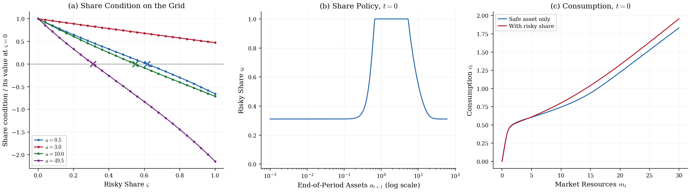

Panel (a) shows the fallback at work. At each asset node the solver has the share condition at the grid shares (the dots). The cross marks where linear interpolation puts its first zero. A curve that stays positive is a corner at $ς = 1$ . In panel (b), a household with modest savings holds only the risky asset, since its future labor income behaves like a safe holding. As savings grow relative to that income, the risky share falls. At the smallest balances it also falls below one. There, next period’s marginal utility is dominated by the zero-wage draw, in which the portfolio is the household’s only resource. Both ends of the policy approach the same share, printed above, because at both ends the portfolio return alone governs next period’s consumption in the states that dominate its marginal utility. Panel (c) and the table below compare consumption with and without the risky asset.

m_show = [1.0, 5.0, 10.0, 20.0, 30.0]
print(
    format_table(
        ["m", "Safe asset only", "With risky share"],
        [[m, f"{sol.consumption_saving.c_func(m):.4f}", f"{psol.consumption_saving.c_func(m):.4f}"] for m in m_show],
    )
)

m     Safe asset only  With risky share
----  ---------------  ----------------
1.0   0.4188           0.4174
5.0   0.6050           0.6090
10.0  0.7443           0.8011
20.0  1.2218           1.3244
30.0  1.8317           1.9561

At low market resources the two consumption functions nearly coincide. At higher resources the higher expected return raises consumption, by more the more the household has saved.