The Health Investment Model with Sequential EGM - The Sequential Endogenous Grid Method

Part A of the Online Appendix tests interpolation methods on a consumption-saving problem with health investment, the model of Ludwig and Schoen (2018) extended with the wage and depreciation risk that White (2015) adds. This notebook first solves it as HARK does. EGM $^{n}$ then splits each period into stages, each one a closed-form inversion, whose last stage produces the curvilinear mesh that ENGINE interpolates. A final part compares the two solutions and reruns two of the archived comparisons.

import sys

sys.path.append("../")
sys.path.append("../figures")

import matplotlib.pyplot as plt
import numpy as np
from cli import format_table
from engine.engine2d import Engine2DInterp, ipm_violations
from figure_styles import apply_engine_style
from generate_grid_transformation import (
    draw_health_grid_transformation,
    get_health_model_grids,
)
from HARK.ConsumptionSaving.ConsHealthModel import eval_marg_health_prod
from HARK.interpolation import Curvilinear2DInterp
from HARK.rewards import CRRAutilityP
from health_model_interpolation_benchmark import (
    POLICY_DIFF_CSV,
    SOLVER_EQUIVALENCE_CSV,
    draw_interpolation_errors,
    interpolation_accuracy,
    policy_diff_rows,
    solved,
    solver_equivalence_rows,
)
from HARKmodels.ConsHealthSeparableModel import (
    BasicHealthConsumerType,
    SequentialHealthConsumerType,
    invert_sequential_stages,
    paper_timing_params,
    post_decision_marginals,
    post_decision_mesh,
)
from HARKmodels.health_interp import HEALTH_CURVATURE_BOUND, HealthEngine2DInterp
from repo_paths import FIG_DIR, read_rows

apply_engine_style()

1The Household Problem¶

Each period the household observes market resources $m_{t}$ and health capital $h_{t}$ , and chooses consumption $c_{t}$ and health investment $n_{t}$ :

\begin{matrix} v_{t} (m_{t}, h_{t}) & = \max_{c_{t} \geq 0, n_{t} \geq 0} u (c_{t}) + β 𝒮_{t} 𝔼_{t} [v_{t + 1} (m_{t + 1}, h_{t + 1})] \\ H_{t} & = h_{t} + g (n_{t}), a_{t} = m_{t} - c_{t} - n_{t}, 𝒮_{t} = 1 - 𝖣_{t} / (1 + H_{t}), \\ h_{t + 1} & = (1 - δ_{t + 1}) H_{t}, m_{t + 1} = 𝖱 a_{t} + ω_{t + 1} H_{t}, \end{matrix}

(1)

with $u (c) = c^{1 - ρ} / (1 - ρ)$ and $g (n) = (γ / ε) n^{ε}$ . Investment builds post-investment health $H_{t}$ , which lowers the probability of death and raises next period’s labor income $ω_{t + 1} H_{t}$ before it depreciates at the random rate $δ_{t + 1}$ . The online appendix’s timing comparison sweeps the number of backward-induction cycles and the grid size around one base point, a $44 \times 50$ grid solved over ten cycles. The calibration below is that base point.

params = paper_timing_params()
hark = BasicHealthConsumerType(**params)
wages = hark.ShockDstn[0].atoms[0]
print(
    format_table(
        ["Parameter", "Code name", "Value"],
        [
            ["Discount factor", "DiscFac", hark.DiscFac],
            ["Relative risk aversion", "CRRA", hark.CRRA],
            ["Interest factor", "Rfree", hark.Rfree[0]],
            ["Health production elasticity", "HealthProdExp", hark.HealthProdExp],
            ["Health production scale", "HealthProdFac", hark.HealthProdFac],
            ["Maximum death probability", "DieProbMax", hark.DieProbMax[0]],
            ["Mean depreciation rate", "DeprRteMean", hark.DeprRteMean[0]],
            ["Smallest wage draw", "", f"{wages.min():.4f}"],
            ["Asset grid nodes", "aXtraCount", hark.aXtraCount],
            ["Extra nodes near zero assets", "aXtraExtra", len(hark.aXtraExtra)],
            ["Health grid nodes", "HLvlGrid", hark.HLvlGrid.size],
            ["Health grid range", "HLvlGrid", f"[{hark.HLvlGrid[0]}, {hark.HLvlGrid[-1]}]"],
            ["Backward-induction cycles", "cycles", params["cycles"]],
        ],
    )
)

Parameter                     Code name      Value
----------------------------  -------------  ------------
Discount factor               DiscFac        0.95
Relative risk aversion        CRRA           0.5
Interest factor               Rfree          1.03
Health production elasticity  HealthProdExp  0.35
Health production scale       HealthProdFac  1.0
Maximum death probability     DieProbMax     0.5
Mean depreciation rate        DeprRteMean    0.05
Smallest wage draw                           0.0850
Asset grid nodes              aXtraCount     44
Extra nodes near zero assets  aXtraExtra     7
Health grid nodes             HLvlGrid       50
Health grid range             HLvlGrid       [0.01, 50.0]
Backward-induction cycles     cycles         10

HARK’s asset grid adds the extra nodes near zero to the regular ones. In the timing table, a grid labelled $44 \times 50$ counts only the regular asset nodes and is the grid of this calibration.

2HARK’s Baseline Solution¶

White (2015) folds the transitions and the risk into the end-of-period value $w_{t} (a_{t}, H_{t}) = β 𝒮_{t} 𝔼_{t} [v_{t + 1}]$ and inverts both first-order conditions at once on a rectangular grid of $(a_{t}, H_{t})$ :

c_{t} = {(w_{t}^{a})}^{- 1 / ρ}, g^{'} (n_{t}) = \frac{w_{t}^{a}}{w_{t}^{H}}, m_{t} = a_{t} + c_{t} + n_{t}, h_{t} = H_{t} - g (n_{t}) .

(2)

The inverted states $(m_{t}, h_{t})$ form a curvilinear mesh, which White interpolates with the sector-walking method HARK implements as Curvilinear2DInterp. BasicHealthConsumerType runs that solver with that interpolant.

hark.solve()
x_hark, y_hark = hark.solution[0].x_values, hark.solution[0].y_values
print(f"periods solved: {len(hark.solution)}")
print(f"endogenous mesh at t = 0: {x_hark.shape[0]} x {x_hark.shape[1]} nodes")

periods solved: 10
endogenous mesh at t = 0: 60 x 50 nodes

Every period’s solution is one interpolant with three outputs: the inverse value $u^{- 1} (v_{t})$ , consumption and health investment. Its nodes at $t = 0$ :

fig, ax = plt.subplots(figsize=(7, 5))
ax.plot(x_hark.ravel(), y_hark.ravel(), ".", color="0.2", ms=2)
ax.set_xlim(0.0, 100.0)
ax.set_ylim(0.0, 50.0)
ax.set_xlabel(r"Market Resources $m_t$")
ax.set_ylabel(r"Health Capital $h_t$")
plt.show()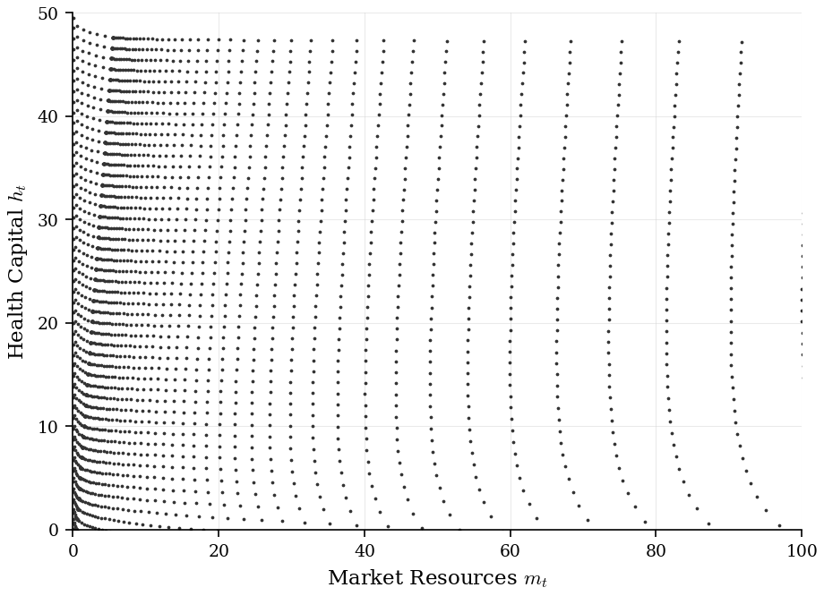

Each near-vertical string of dots is one asset node traced across the health grid. At low post-investment health the inversion assigns more investment, which maps the same asset node to more market resources and less beginning health. Every string therefore bends to the right as health falls. Nodes crowd near $m_{t} = 0$ , where the asset grid is densest.

Below are cross-sections of the two policies at health capital $h_{t} = 20$ .

m_line = np.linspace(0.0, 20.0, 400)
h_line = np.full_like(m_line, 20.0)
_, c_hark, n_hark = hark.solution[0](m_line, h_line)

fig, ax = plt.subplots(figsize=(7, 4.5))
ax.plot(m_line, c_hark, label=r"Consumption $c_t$")
ax.plot(m_line, n_hark, label=r"Health Investment $n_t$")
ax.set_xlabel(r"Market Resources $m_t$")
ax.legend()
plt.show()

kink_row = 1 + hark.constrained_N  # the zero-asset row of the mesh
m_kink = np.interp(20.0, y_hark[kink_row], x_hark[kink_row])
print(f"at h = 20, the zero-asset mesh line lies at m = {m_kink:.2f}")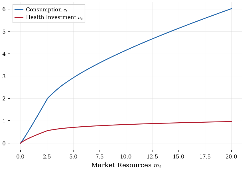

at h = 20, the zero-asset mesh line lies at m = 2.58

Both policies rise with market resources. The kink at the printed value of $m_{t}$ marks where the household starts to save. Below it the liquidity constraint binds. Every additional unit of resources then goes to consumption or investment. Investment stays positive at every $m_{t} > 0$ , since the marginal product $g^{'} (n)$ grows without bound as $n \to 0$ .

3The Stage Decomposition¶

EGM $^{n}$ splits the period into three stages, each solved by one inversion. Following the online appendix, $v_{t}^{0} \equiv v_{t}$ denotes the value at the first decision stage and $v_{t}^{1}$ the value once investment is chosen.

The post-decision stage values the end-of-period states, $w_{t} (a_{t}, H_{t})$ , together with its marginals $w_{t}^{a}$ and $w_{t}^{H}$ .
The consumption stage solves $v_{t}^{1} (ℓ_{t}, H_{t}) = \max_{c_{t}} u (c_{t}) + w_{t} (ℓ_{t} - c_{t}, H_{t})$ . For each fixed $H_{t}$ this is a standard consumption-saving problem: $c_{t} = {(w_{t}^{a})}^{- 1 / ρ}$ and liquid wealth $ℓ_{t} = a_{t} + c_{t}$ .
The health investment stage solves $v_{t}^{0} (m_{t}, h_{t}) = \max_{n_{t}} v_{t}^{1} (m_{t} - n_{t}, h_{t} + g (n_{t}))$ . Its first-order condition $g^{'} (n_{t}) = {(v_{t}^{1})}^{ℓ} / {(v_{t}^{1})}^{H}$ inverts in closed form. The transitions then return $m_{t} = ℓ_{t} + n_{t}$ and $h_{t} = H_{t} - g (n_{t})$ .

SequentialHealthConsumerType keeps each stage as its own interpolant. Run here with ENGINE:

egmn = SequentialHealthConsumerType(interpolator=HealthEngine2DInterp, **params)
egmn.solve()
sol = egmn.solution[0]
for name in ("post_decision", "consumption", "health_investment"):
    print(f"{name:18s} {type(getattr(sol, name).interp).__name__}")

post_decision      Engine2DInterp
consumption        Engine2DInterp
health_investment  Engine2DInterp

The first two stages are defined on the rectangular $(a, H)$ grid. Only the last one, which maps to the decision-time states $(m, h)$ , needs curvilinear interpolation.

The cell below solves the model again at the default margin. It compares every period’s mesh and the policies at a grid of off-mesh points with the matched-margin solution.

print(f"search margin used for the health meshes: {HEALTH_CURVATURE_BOUND}")
default = SequentialHealthConsumerType(interpolator=Engine2DInterp, **params)
default.solve()
same_mesh = all(
    np.array_equal(a.health_investment.interp.fx, b.health_investment.interp.fx)
    and np.array_equal(a.health_investment.interp.fy, b.health_investment.interp.fy)
    for a, b in zip(egmn.solution, default.solution, strict=True)
)
m_q, h_q = np.meshgrid(np.linspace(0.5, 25.0, 50), np.linspace(0.5, 25.0, 40), indexing="ij")
same_policy = all(
    np.array_equal(x, y) for x, y in zip(sol(m_q, h_q), default.solution[0](m_q, h_q), strict=True)
)
print(f"default margin 2: identical meshes in all periods: {same_mesh}")
print(f"default margin 2: identical policies at t = 0:      {same_policy}")

search margin used for the health meshes: 16

default margin 2: identical meshes in all periods: True
default margin 2: identical policies at t = 0:      True

Every Stage in Closed Form¶

The solver’s stage functions are ordinary module functions, which this notebook calls directly. Rebuilding the post-decision marginals at $t = 0$ from next period’s solution and applying the two inversions reproduces the mesh ENGINE interpolates. Both first-order conditions hold at every node.

constrained, a_mat, H_mat = post_decision_mesh(egmn.aLvlGrid, egmn.HLvlGrid, egmn.ShockDstn[0])
rho, eps, gam = egmn.CRRA, egmn.HealthProdExp, egmn.HealthProdFac
w, w_a, w_H = post_decision_marginals(
    egmn.solution[1],
    egmn.ShockDstn[0],
    a_mat,
    H_mat,
    (egmn.Rfree[0], rho, eps, gam),
    egmn.DieProbMax[0],
    egmn.DiscFac,
)
c, ell, n, m, h = invert_sequential_stages(w_a, w_H, a_mat, H_mat, rho, eps, gam)

mesh = sol.health_investment.interp
interior = slice(1 + egmn.constrained_N, None)  # below: the m = 0 row and the constrained rows
print(f"max |u'(c) / w_a - 1|        = {np.max(np.abs(CRRAutilityP(c, rho) / w_a - 1)):.1e}")
print(f"max |g'(n) w_H / w_a - 1|    = {np.max(np.abs(eval_marg_health_prod(n, eps, gam) * w_H / w_a - 1)):.1e}")
print(f"max |m - ENGINE mesh m|      = {np.max(np.abs(mesh.fx[interior] - m)):.1e}")
print(f"max |h - ENGINE mesh h|      = {np.max(np.abs(mesh.fy[interior] - h)):.1e}")

max |u'(c) / w_a - 1|        = 2.2e-16
max |g'(n) w_H / w_a - 1|    = 4.4e-16
max |m - ENGINE mesh m|      = 0.0e+00
max |h - ENGINE mesh h|      = 0.0e+00

The investment stage works on the consumption stage’s own nodes $(ℓ, H)$ , where the envelope conditions give ${(v_{t}^{1})}^{ℓ} = u^{'} (c_{t}) = w_{t}^{a}$ and ${(v_{t}^{1})}^{H} = w_{t}^{H}$ . No interpolation therefore separates the two inversions. Because every wage draw is positive (the calibration table prints the smallest), a household can end the period with no assets. Beneath the inverted nodes, the solver adds constrained_N liquidity-constrained rows at $a = 0$ and a row at $m = 0$ .

The Endogenous Mesh¶

The paper’s grid-transformation figure, redrawn below on its $25 \times 20$ grid for a two-period model, shows the map from the regular post-decision grid to the curvilinear decision-time mesh:

fig = draw_health_grid_transformation(get_health_model_grids())
plt.show()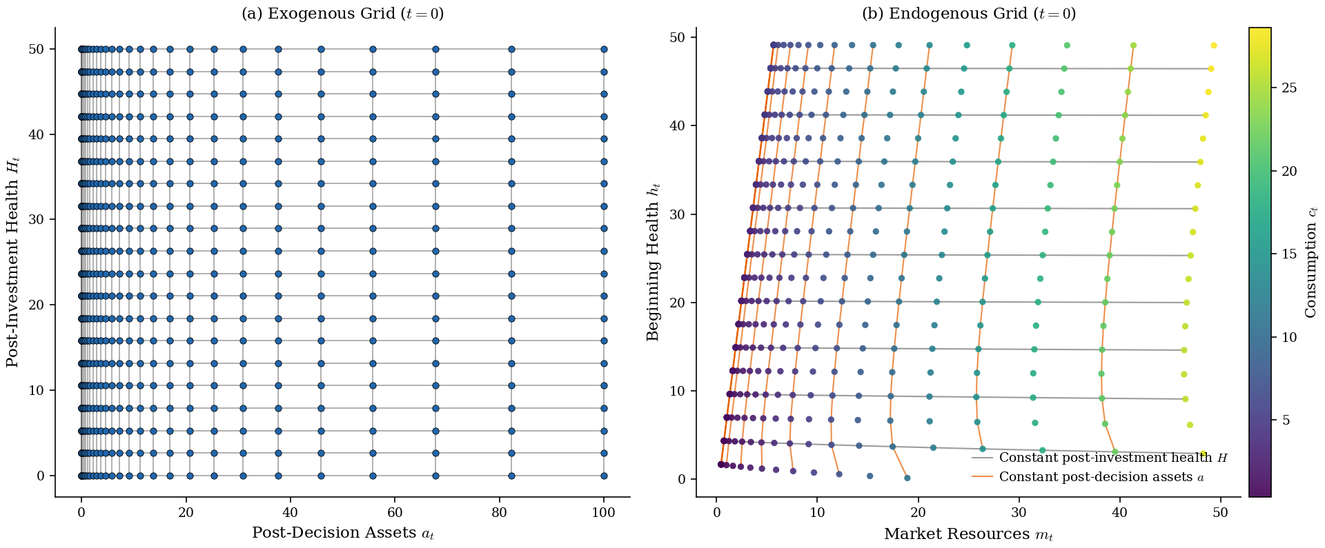

Lines of constant post-investment health and constant assets keep their order through the warp, the index-monotone property (IPM) ENGINE requires. The check below runs on every period’s mesh of the ten-cycle solution.

rows = []
for t, sol_t in enumerate(egmn.solution):
    x, y = sol_t.health_investment.interp.fx, sol_t.health_investment.interp.fy
    rows.append([t, sum(ipm_violations(x, y))])
print(format_table(["t", "IPM breaks"], rows))

t  IPM breaks
-  ----------
0  0
1  0
2  0
3  0
4  0
5  0
6  0
7  0
8  0
9  0

Every mesh satisfies IPM.

4Comparing the Two Solutions¶

The Same Inversion¶

Given the same interpolant, the two solvers perform the same inversions on the same grid. The archive tests this on its small accuracy grid, where solver_equivalence_rows solves the model both ways under HARK’s curvilinear interpolant and measures the gap between the two sets of policies at off-mesh points; health_solver_equivalence.csv stores the result. Rerunning the check reproduces the file.

def compare_to_csv(path, rows, n_keys=1):
    """Print freshly computed rows beside the committed CSV at ``path``; the
    first ``n_keys`` columns label each row and must match the file's.
    """
    published = read_rows(path)
    header = list(published[0])
    table = []
    for row, pub in zip(rows, published, strict=True):
        key = [pub[col] for col in header[:n_keys]]
        if row[:n_keys] != key:
            raise ValueError(f"row {row[:n_keys]} does not match published row {key}")
        table += [
            [" ".join([*key, col]), value, pub[col]]
            for col, value in zip(header[n_keys:], row[n_keys:], strict=True)
        ]
    print(format_table(["Reading", "This run", "Published"], table))


compare_to_csv(SOLVER_EQUIVALENCE_CSV, solver_equivalence_rows())

Reading     This run   Published
----------  ---------  ---------
c abs_mean  1.228e-14  1.289e-14
c abs_max   2.611e-13  2.931e-13
n abs_mean  5.235e-17  5.757e-17
n abs_max   1.221e-15  8.882e-16

The largest absolute gap in consumption is below 10^-12, rounding error.

Because the solvers agree, any difference between two solutions computed at the same grid comes from the interpolant alone.

Three Interpolants¶

The archive’s second check holds the simultaneous solver fixed and runs each interpolant inside its own backward solve: White’s curvilinear method, ENGINE and Delaunay triangulation, which Ludwig and Schoen (2018) introduced on the version of this model whose only risk is survival. On a uniform $50 \times 40$ grid of off-mesh points spanning $m, h \in [0.5, 25]$ , it measures each method’s relative policy difference from the curvilinear solution, stored in health_interp_policy_diff.csv. Rerun here:

accuracy = interpolation_accuracy()
compare_to_csv(POLICY_DIFF_CSV, policy_diff_rows(accuracy), n_keys=2)

Reading              This run   Published
-------------------  ---------  ---------
engine c rel_mean    5.754e-05  5.754e-05
engine c rel_max     7.161e-03  7.161e-03
engine c n_valid     2000       2000
engine n rel_mean    1.783e-03  1.783e-03
engine n rel_max     4.782e-02  4.782e-02
engine n n_valid     2000       2000
delaunay c rel_mean  3.530e-04  3.530e-04
delaunay c rel_max   1.461e-01  1.461e-01
delaunay c n_valid   2000       2000
delaunay n rel_mean  4.920e-03  4.920e-03
delaunay n rel_max   3.513e-01  3.513e-01
delaunay n n_valid   2000       2000

The paper’s error map draws the consumption difference over the query plane:

fig = draw_interpolation_errors(accuracy)
reference = solved(BasicHealthConsumerType, Curvilinear2DInterp).solution[0]
kink_row = 1 + egmn.constrained_N  # the zero-asset row of the mesh
for ax in fig.axes[:2]:
    limits = ax.get_xlim(), ax.get_ylim()
    ax.plot(
        reference.x_values[kink_row],
        reference.y_values[kink_row],
        color="black",
        lw=1.0,
        ls="--",
        label="Zero-Asset Mesh Line",
    )
    ax.set_xlim(limits[0])
    ax.set_ylim(limits[1])
fig.axes[0].legend(loc="lower right", fontsize=8)
plt.show()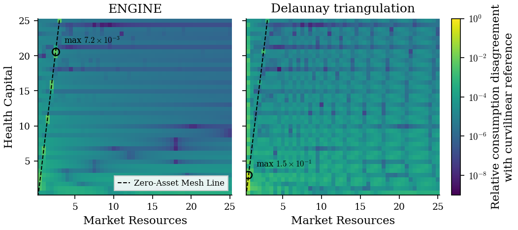

ENGINE stays close to the curvilinear solution over most of the plane. Its largest differences lie in a few spots at low market resources, all on the dashed mesh line of zero assets, where the liquidity constraint stops binding and the policies kink. The triangulation’s differences are larger and cover the whole plane, with its maximum at the lowest market resources.

Solve Times¶

Timings depend on the machine, so this page reads the published measurements from health_model_summary.csv instead of timing the solves during the build. Each cell is the mean of ten timed solves.

summary = {}
for r in read_rows(FIG_DIR / "health_model_summary.csv"):
    summary.setdefault((r["sweep"], r["label"]), {})[r["series"]] = float(r["mean_s"])

rows = []
for (sweep, label), s in summary.items():
    base = s["HARK baseline"]
    point = f"{label} cycles, 44x50 grid" if sweep == "cycles" else f"{label} grid, 10 cycles"
    egmn_s = s["EGM$^n$ + ENGINE"]
    rows.append([point, f"{base:.3f}", f"{egmn_s:.3f} ({base / egmn_s:.1f}x)"])
print(format_table(["Configuration", "Simultaneous + curvilinear", "EGM^n + ENGINE"], rows))

Configuration           Simultaneous + curvilinear  EGM^n + ENGINE
----------------------  --------------------------  --------------
2 cycles, 44x50 grid    0.037                       0.013 (2.8x)
5 cycles, 44x50 grid    0.131                       0.033 (4.0x)
10 cycles, 44x50 grid   0.296                       0.071 (4.2x)
15 cycles, 44x50 grid   0.460                       0.103 (4.4x)
20x15 grid, 10 cycles   0.044                       0.014 (3.1x)
44x50 grid, 10 cycles   0.296                       0.071 (4.2x)
88x50 grid, 10 cycles   0.559                       0.126 (4.4x)
132x50 grid, 10 cycles  0.860                       0.191 (4.5x)
176x50 grid, 10 cycles  1.162                       0.247 (4.7x)

Times are in seconds. The ratio in parentheses is the curvilinear baseline’s time over that of EGM $^{n}$ with ENGINE, which solves the model 2.8 to 4.7 times faster across both sweeps.